Dimensionality Reduction Principal component Analysis Introduction23 1 Vector

Dimensionality Reduction Principal component Analysis

• • Introduction(23. 1) Vector space Model-Term document matrix(23. 1. 2) Precision and Recall(23. 1. 4) Features – Identification – Selection • Dimension Reduction – Principal Component analysis • • Latent Semantic Indexing. Plagiarism Cross language retrieval Query Expansion

Examples of data intensive scenario • Casinos are capturing data using cameras and tracking each and every move of their customers. • Your smart phone apps collects a lot of personal details about you • Your set top box collects data about which programs preferences and timings

What are Dimension Reduction techniques? • Dimension Reduction refers to the process of converting a set of data having vast dimensions into data with lesser dimensions • Ensuring that it conveys similar information concisely.

Feature selection Vs. Dimension reduction • Feature Selection – Feature selection yields a subset of features from the original set of features, which are best representatives of the data. – It is an exhaustive search. – Feature selection is done in the context of an optimization problem. • Dimension Reduction – Dimensionality reduction is generic – Depends on the data and not on what you plan to do with it. – Not interested in how algorithm works • Classification problem • you select the features that will help you classify your data better • dimensionality reduction algorithm is unaware of this and just projects the data into a lower dimensionality space.

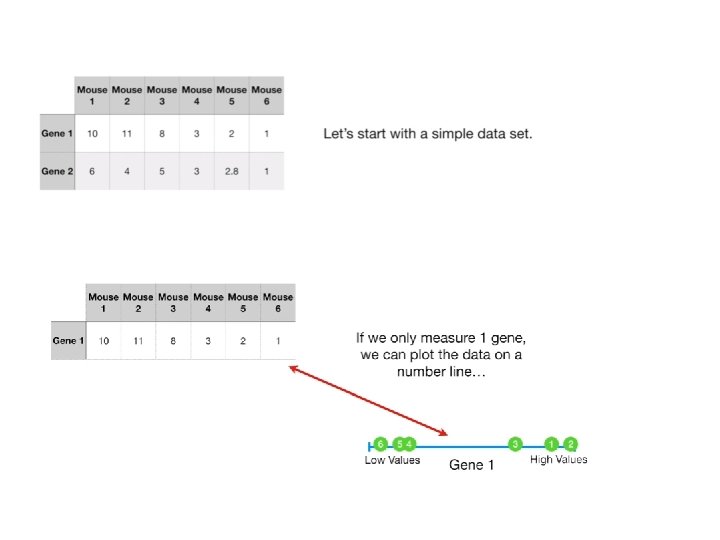
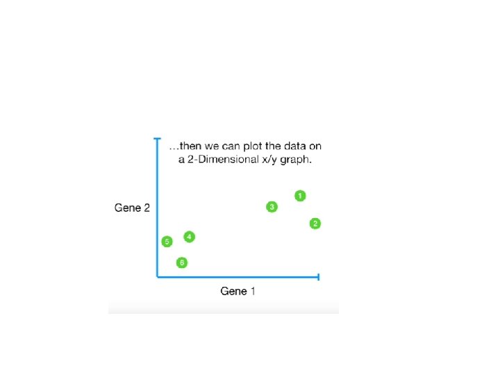
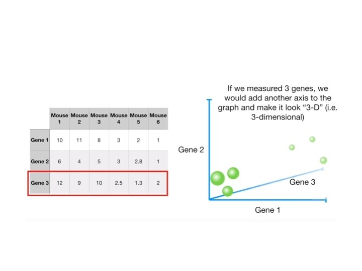
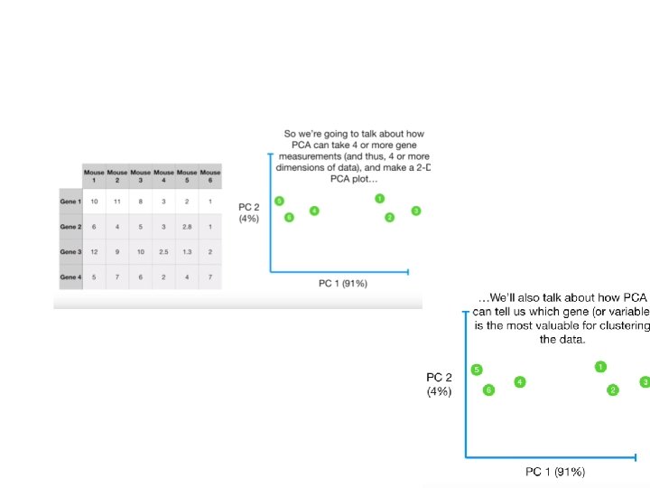
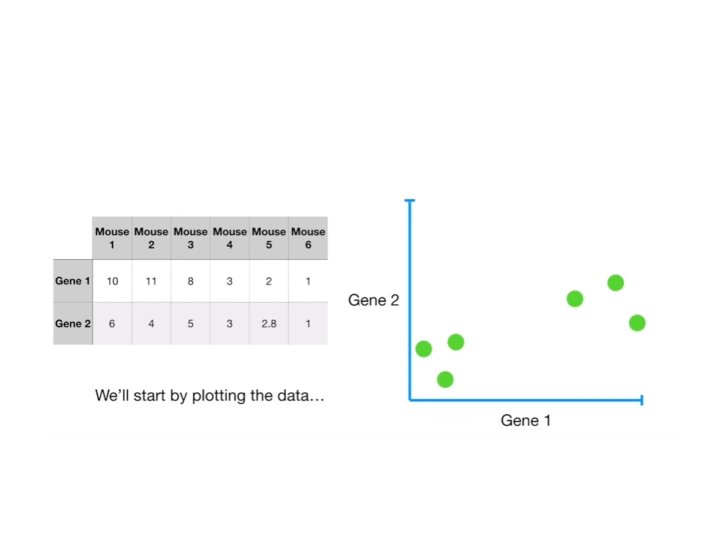
Why? • It helps in data compressing and reducing the storage space required • Less dimensions leads to less computing • It takes care of multi-collinearity that improves the model performance. • It removes redundant features. • Reducing the dimensions of data to 2 D or 3 D may allow us to plot and visualize it precisely.

PCA using Singular value Decomposition

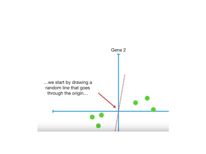
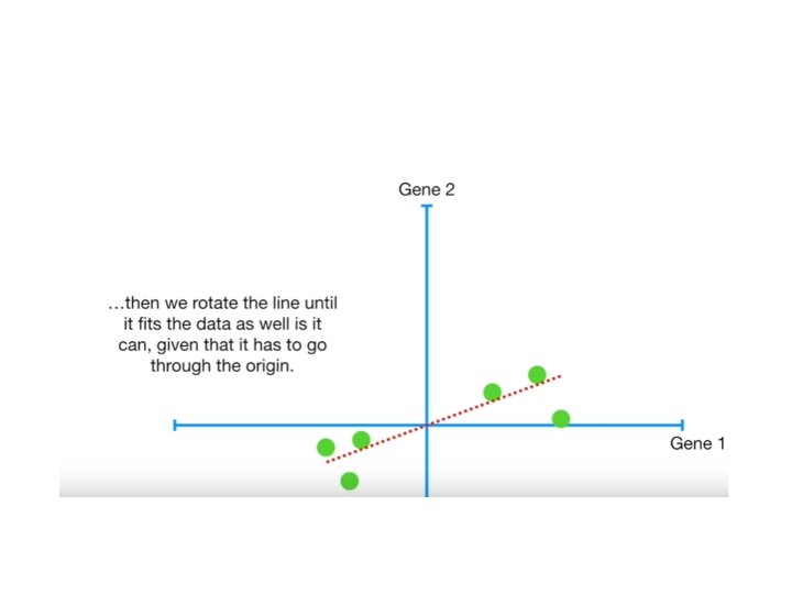
BUT HOW DOES PCA DECIDES WHICH LINE FITS THE BEST?

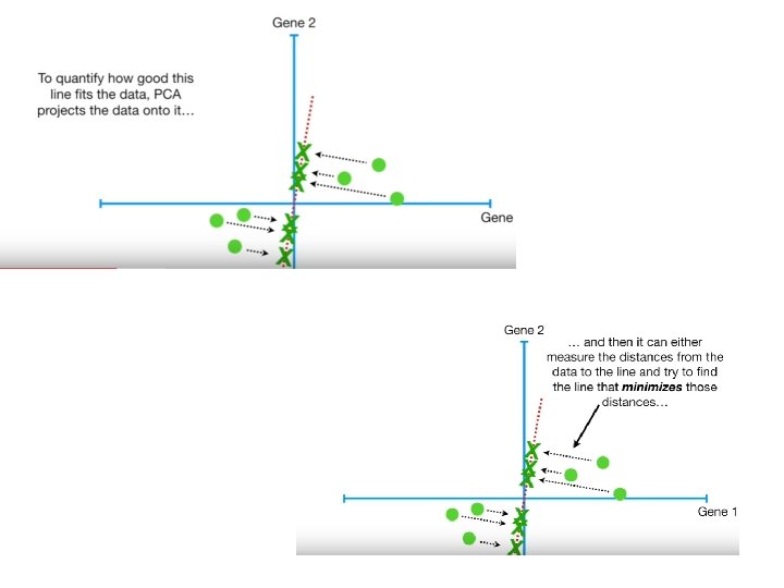
• D 1 ->distance from point x 1 to origin • d 2>->distance from point x 2 to origin • D 3 ->distance from point x 3 to origin • D 4 ->distance from point x 4 to origin • D 5 ->distance from point x 5 to origin • D 6 ->distance from point x 6 to origin

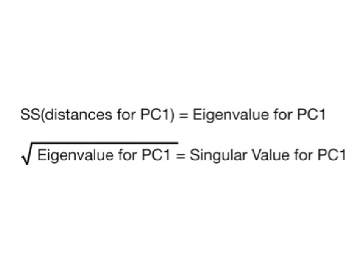
• Continue the same for all possible line • Repeat it until we get a line with largest possible ss(distance) • This line is called principal Component(PC 1).

• Pc 1 has slope 0. 25. • That means is spread along X axis(Gene-1) • The ss(distance)of best fit line is called as Eigenvalue of PC 1