Dimensionality reduction PCA SVD MDS ICA and friends

Dimensionality reduction PCA, SVD, MDS, ICA, and friends Jure Leskovec Machine Learning recitation April 27 2006

Why dimensionality reduction? n n n Some features may be irrelevant We want to visualize high dimensional data “Intrinsic” dimensionality may be smaller than the number of features

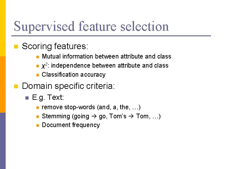
Supervised feature selection n Scoring features: n n Mutual information between attribute and class χ2: independence between attribute and class Classification accuracy Domain specific criteria: n E. g. Text: n n n remove stop-words (and, a, the, …) Stemming (going go, Tom’s Tom, …) Document frequency

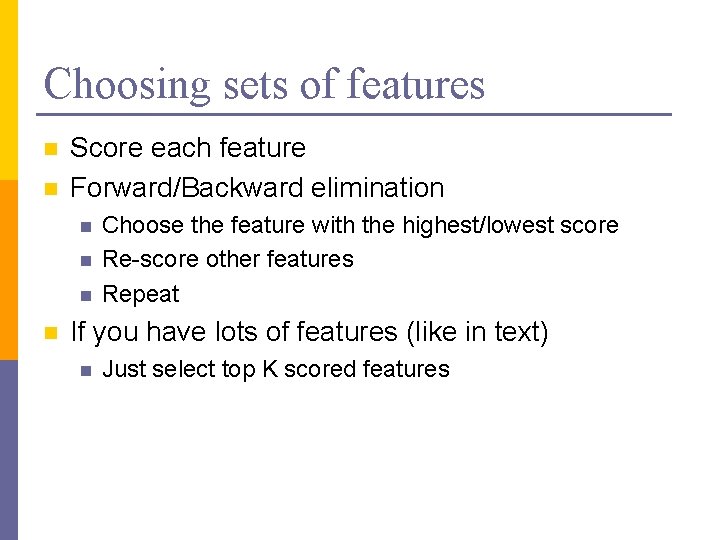
Choosing sets of features n n Score each feature Forward/Backward elimination n n Choose the feature with the highest/lowest score Re-score other features Repeat If you have lots of features (like in text) n Just select top K scored features

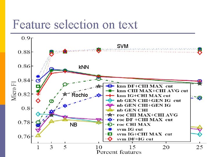
Feature selection on text SVM k. NN Rochio NB

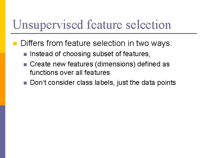
Unsupervised feature selection n Differs from feature selection in two ways: n n n Instead of choosing subset of features, Create new features (dimensions) defined as functions over all features Don’t consider class labels, just the data points

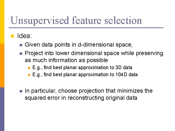
Unsupervised feature selection n Idea: n n Given data points in d-dimensional space, Project into lower dimensional space while preserving as much information as possible n n n E. g. , find best planar approximation to 3 D data E. g. , find best planar approximation to 104 D data In particular, choose projection that minimizes the squared error in reconstructing original data

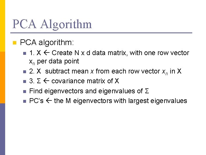
PCA Algorithm n PCA algorithm: n n n 1. X Create N x d data matrix, with one row vector xn per data point 2. X subtract mean x from each row vector xn in X 3. Σ covariance matrix of X Find eigenvectors and eigenvalues of Σ PC’s the M eigenvectors with largest eigenvalues

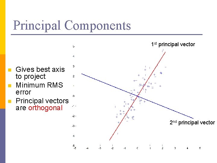
PCA Algorithm in Matlab % generate data Data = mvnrnd([5, 5], [1 1. 5; 1. 5 3], 100); figure(1); plot(Data(: , 1), Data(: , 2), '+'); %center the data for i = 1: size(Data, 1) Data(i, : ) = Data(i, : ) - mean(Data); end Data. Cov = cov(Data); %covariance matrix [PC, variances, explained] = pcacov(Data. Cov); %eigen % plot principal components figure(2); clf; hold on; plot(Data(: , 1), Data(: , 2), '+b'); plot(PC(1, 1)*[-5 5], PC(2, 1)*[-5 5], '-r’) plot(PC(1, 2)*[-5 5], PC(2, 2)*[-5 5], '-b’); hold off % project down to 1 dimension Pca. Pos = Data * PC(: , 1);

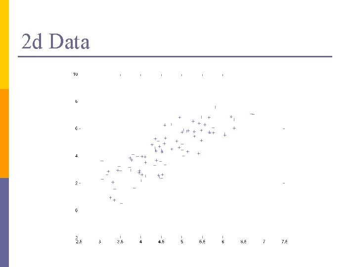
2 d Data

Principal Components 1 st principal vector n n n Gives best axis to project Minimum RMS error Principal vectors are orthogonal 2 nd principal vector

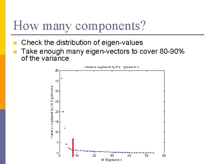
How many components? n n Check the distribution of eigen-values Take enough many eigen-vectors to cover 80 -90% of the variance

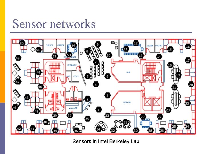
Sensor networks Sensors in Intel Berkeley Lab

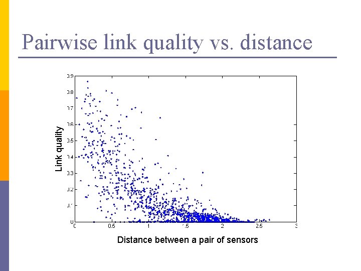
Link quality Pairwise link quality vs. distance Distance between a pair of sensors

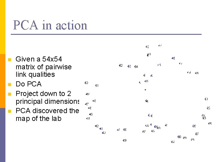
PCA in action n n Given a 54 x 54 matrix of pairwise link qualities Do PCA Project down to 2 principal dimensions PCA discovered the map of the lab

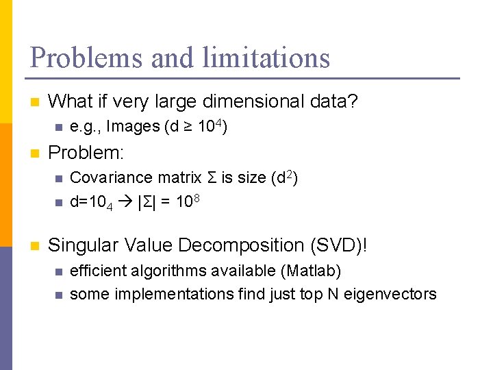
Problems and limitations n What if very large dimensional data? n n Problem: n n n e. g. , Images (d ≥ 104) Covariance matrix Σ is size (d 2) d=104 |Σ| = 108 Singular Value Decomposition (SVD)! n n efficient algorithms available (Matlab) some implementations find just top N eigenvectors

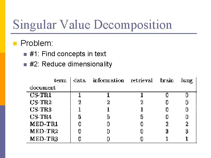
Singular Value Decomposition n Problem: n n #1: Find concepts in text #2: Reduce dimensionality

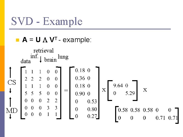
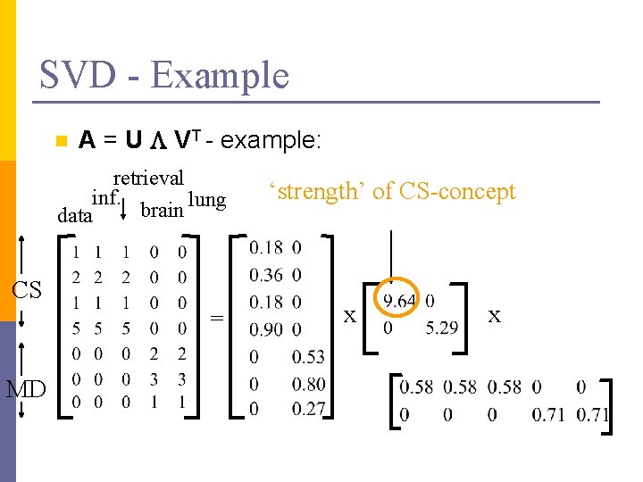
SVD - Definition A[n x m] = U[n x r] L [ r x r] (V[m x r])T n n A: n x m matrix (e. g. , n documents, m terms) U: n x r matrix (n documents, r concepts) L: r x r diagonal matrix (strength of each ‘concept’) (r: rank of the matrix) V: m x r matrix (m terms, r concepts)

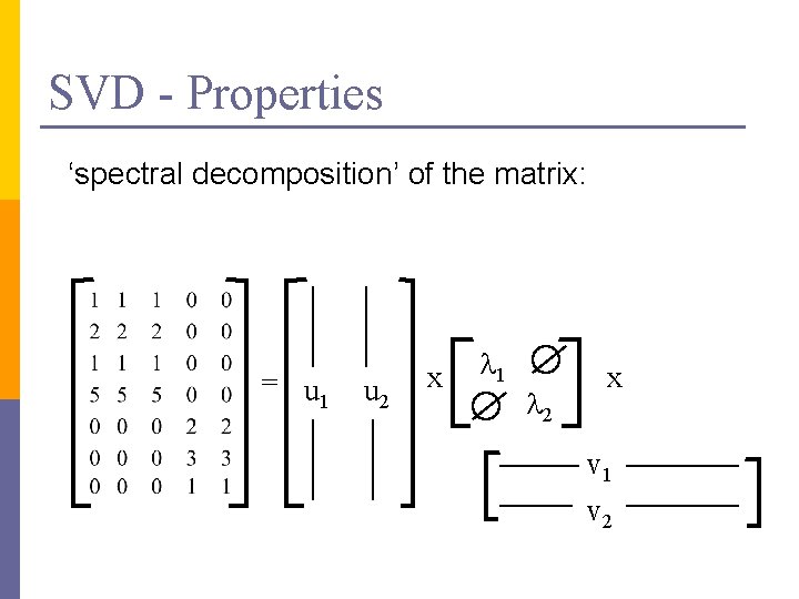
SVD - Properties THEOREM [Press+92]: always possible to decompose matrix A into A = U L VT , where n U, L, V: unique (*) n U, V: column orthonormal (ie. , columns are unit vectors, orthogonal to each other) n n UTU = I; VTV = I (I: identity matrix) L: singular value are positive, and sorted in decreasing order

SVD - Properties ‘spectral decomposition’ of the matrix: = u 1 u 2 x l 1 l 2 x v 1 v 2

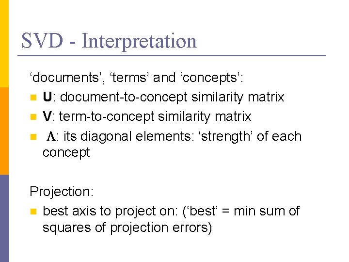
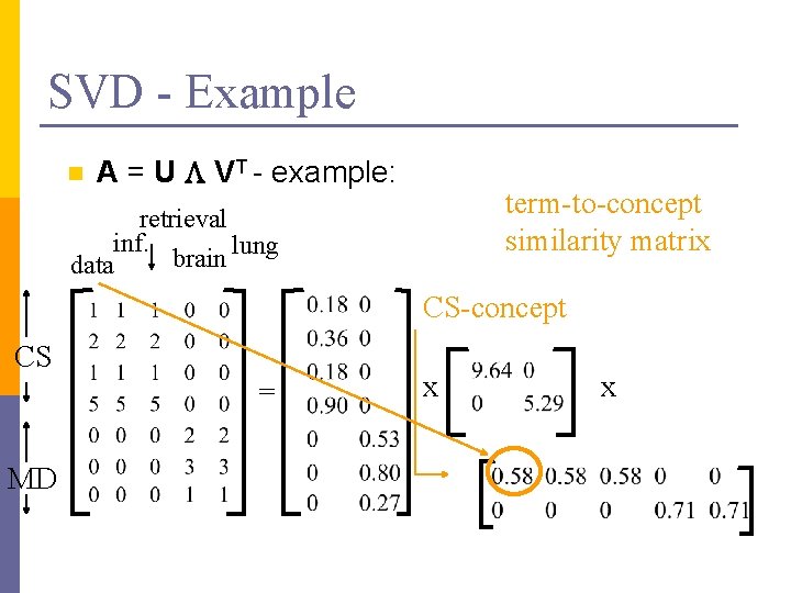
SVD - Interpretation ‘documents’, ‘terms’ and ‘concepts’: n U: document-to-concept similarity matrix n V: term-to-concept similarity matrix n L: its diagonal elements: ‘strength’ of each concept Projection: n best axis to project on: (‘best’ = min sum of squares of projection errors)

SVD - Example n A = U L VT - example: retrieval inf. lung brain data CS = MD x x

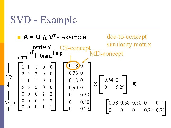
SVD - Example n doc-to-concept similarity matrix retrieval CS-concept inf. MD-concept brain lung A = U L VT - example: data CS = MD x x

SVD - Example n A = U L VT - example: retrieval inf. lung brain data CS = MD ‘strength’ of CS-concept x x

SVD - Example n A = U L VT - example: term-to-concept similarity matrix retrieval inf. lung brain data CS-concept CS = MD x x

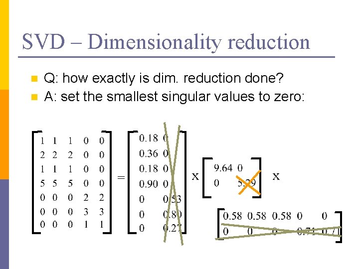
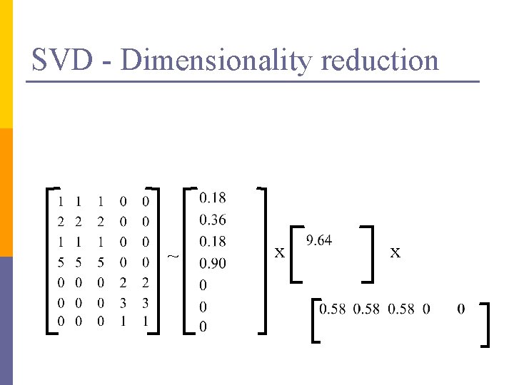
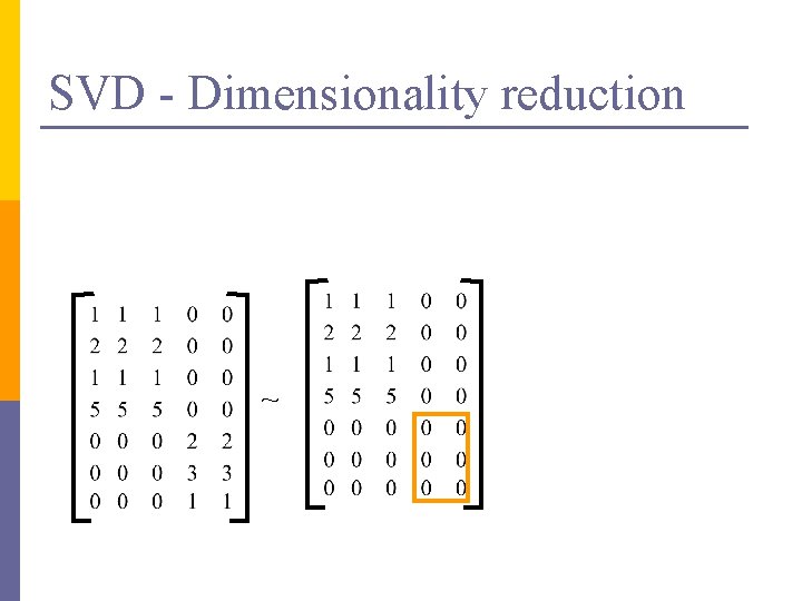
SVD – Dimensionality reduction n n Q: how exactly is dim. reduction done? A: set the smallest singular values to zero: = x x

SVD - Dimensionality reduction ~ x x

SVD - Dimensionality reduction ~

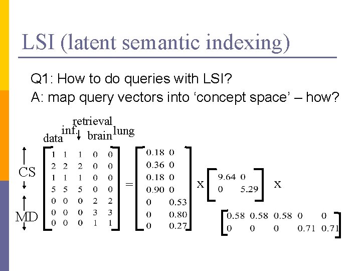
LSI (latent semantic indexing) Q 1: How to do queries with LSI? A: map query vectors into ‘concept space’ – how? retrieval inf. brain lung data CS MD = x x

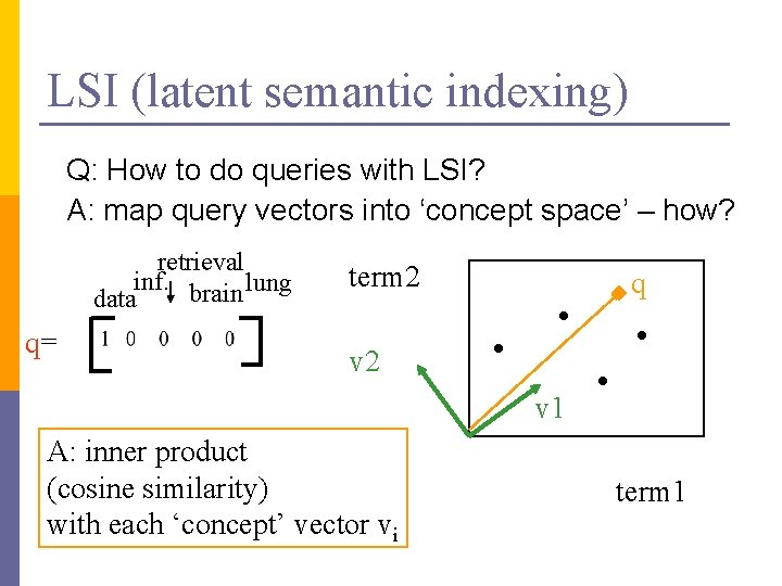
LSI (latent semantic indexing) Q: How to do queries with LSI? A: map query vectors into ‘concept space’ – how? retrieval inf. brain lung data q= term 2 q v 2 v 1 A: inner product (cosine similarity) with each ‘concept’ vector vi term 1

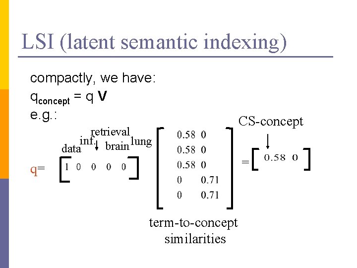
LSI (latent semantic indexing) compactly, we have: qconcept = q V e. g. : retrieval inf. brain lung data q= term-to-concept similarities CS-concept =

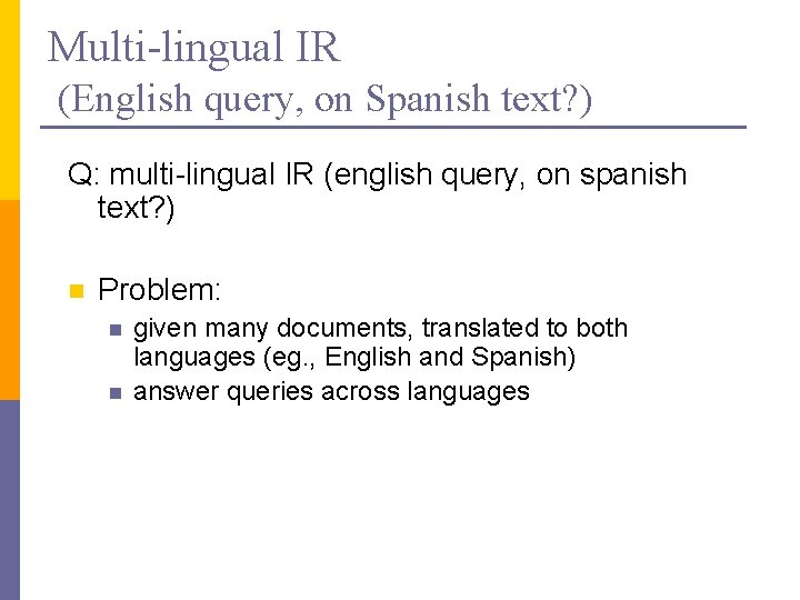
Multi-lingual IR (English query, on Spanish text? ) Q: multi-lingual IR (english query, on spanish text? ) n Problem: n n given many documents, translated to both languages (eg. , English and Spanish) answer queries across languages

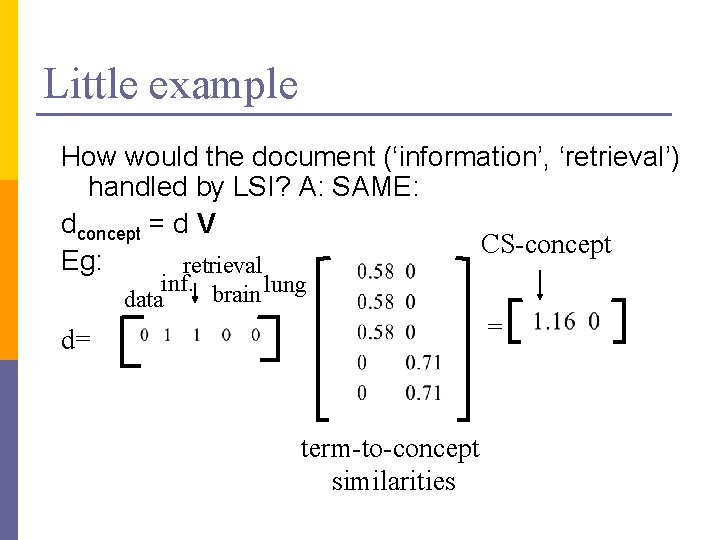
Little example How would the document (‘information’, ‘retrieval’) handled by LSI? A: SAME: dconcept = d V CS-concept Eg: retrieval inf. brain lung data = d= term-to-concept similarities

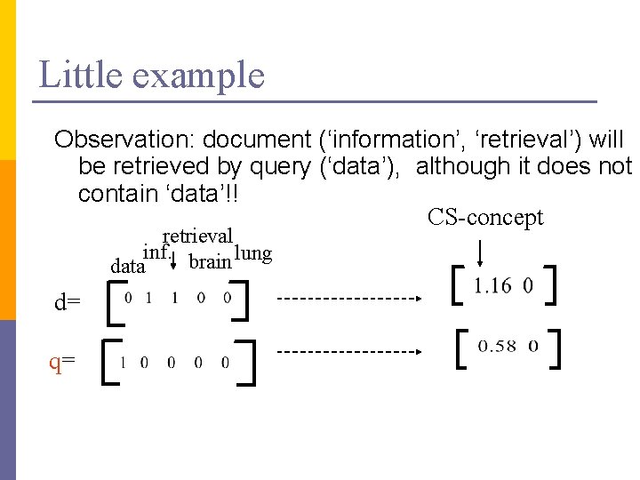
Little example Observation: document (‘information’, ‘retrieval’) will be retrieved by query (‘data’), although it does not contain ‘data’!! CS-concept retrieval inf. brain lung data d= q=

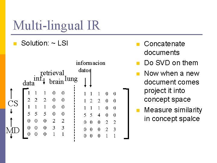
Multi-lingual IR n Solution: ~ LSI n informacion datos retrieval inf. brain lung data CS MD n n n Concatenate documents Do SVD on them Now when a new document comes project it into concept space Measure similarity in concept spalce

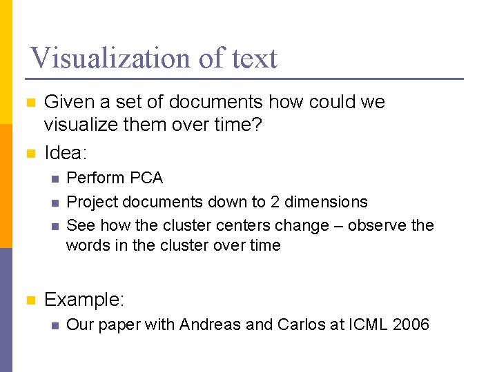
Visualization of text n n Given a set of documents how could we visualize them over time? Idea: n n Perform PCA Project documents down to 2 dimensions See how the cluster centers change – observe the words in the cluster over time Example: n Our paper with Andreas and Carlos at ICML 2006

eigenvectors and eigenvalues on graphs Spectral graph partitioning Spectral clustering Google’s Page. Rank

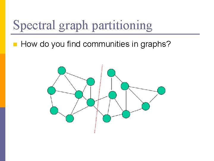
Spectral graph partitioning n How do you find communities in graphs?

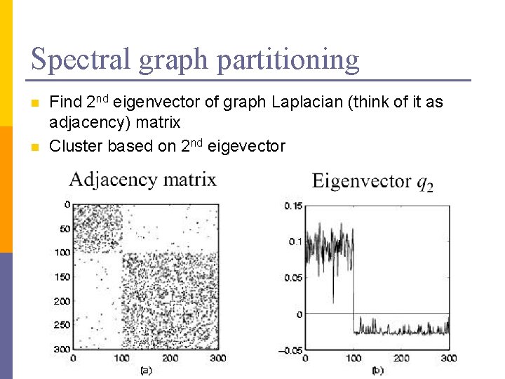
Spectral graph partitioning n n Find 2 nd eigenvector of graph Laplacian (think of it as adjacency) matrix Cluster based on 2 nd eigevector

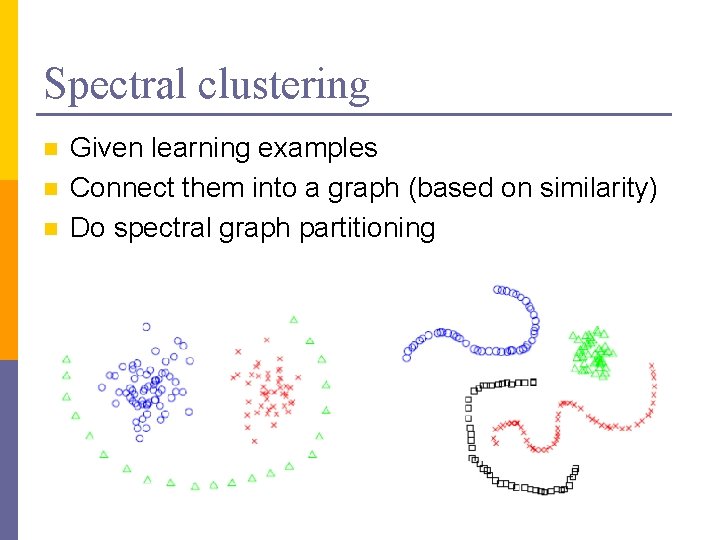
Spectral clustering n n n Given learning examples Connect them into a graph (based on similarity) Do spectral graph partitioning

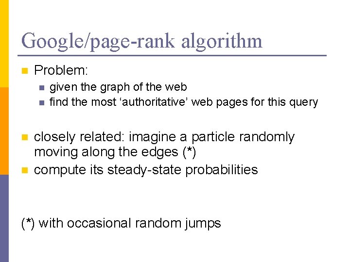
Google/page-rank algorithm n Problem: n n given the graph of the web find the most ‘authoritative’ web pages for this query closely related: imagine a particle randomly moving along the edges (*) compute its steady-state probabilities (*) with occasional random jumps

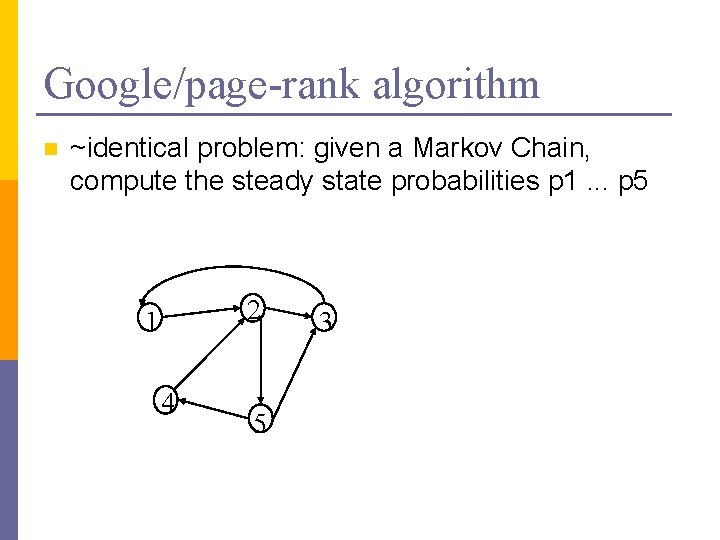
Google/page-rank algorithm n ~identical problem: given a Markov Chain, compute the steady state probabilities p 1. . . p 5 2 1 4 5 3

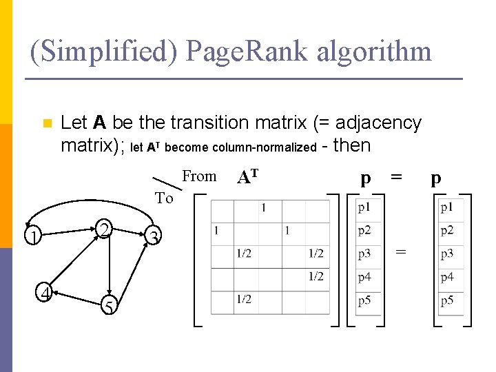
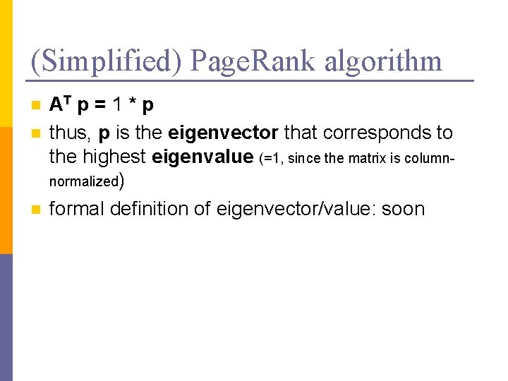
(Simplified) Page. Rank algorithm n Let A be the transition matrix (= adjacency matrix); let AT become column-normalized - then From AT p = To 2 1 4 5 3 = p

(Simplified) Page. Rank algorithm n n n AT p = 1 * p thus, p is the eigenvector that corresponds to the highest eigenvalue (=1, since the matrix is columnnormalized) formal definition of eigenvector/value: soon

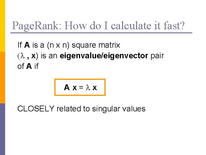
Page. Rank: How do I calculate it fast? If A is a (n x n) square matrix (l , x) is an eigenvalue/eigenvector pair of A if Ax=lx CLOSELY related to singular values

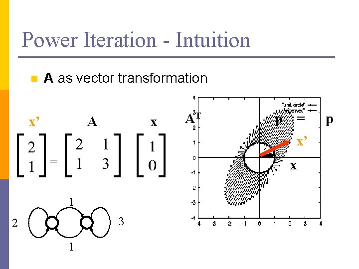
Power Iteration - Intuition n A as vector transformation x’ x A AT p = x’ = x 1 3 2 1 p

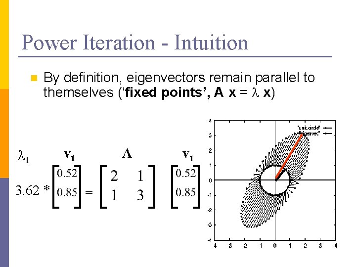
Power Iteration - Intuition n By definition, eigenvectors remain parallel to themselves (‘fixed points’, A x = l x) l 1 3. 62 * v 1 A = v 1

Many PCA-like approaches n Multi-dimensional scaling (MDS): n n n Given a matrix of distances between features We want a lower-dimensional representation that best preserves the distances Independent component analysis (ICA): n Find directions that are most statistically independent

Acknowledgements n Some of the material is borrowed from lectures of Christos Faloutsos and Tom Mitchell