DIMENSIONALITY REDUCTION FOR KMEANS CLUSTERING AND LOW RANK

DIMENSIONALITY REDUCTION FOR K-MEANS CLUSTERING AND LOW RANK APPROXIMATION Michael Cohen, Sam Elder, Cameron Musco, Christopher Musco, and Madalina Persu

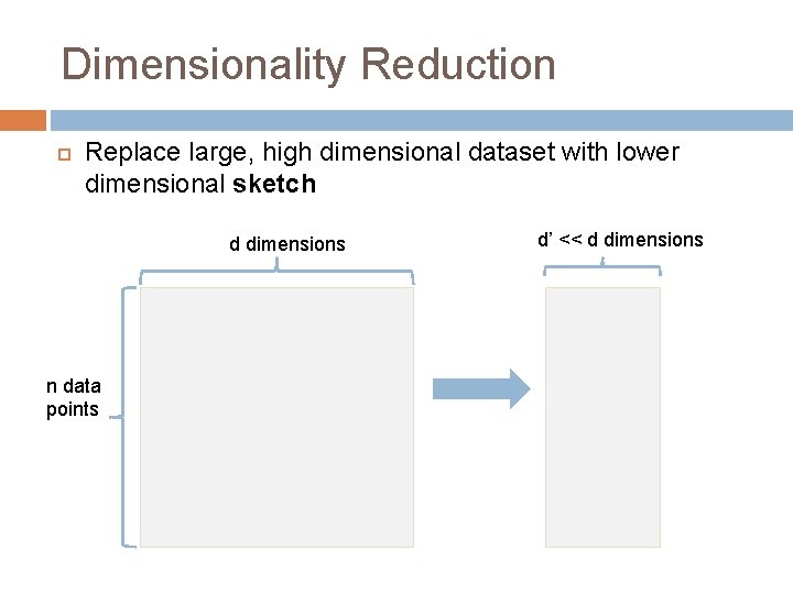
Dimensionality Reduction Replace large, high dimensional dataset with lower dimensional sketch d dimensions n data points d’ << d dimensions

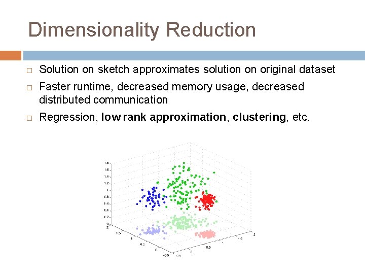
Dimensionality Reduction Solution on sketch approximates solution on original dataset Faster runtime, decreased memory usage, decreased distributed communication Regression, low rank approximation, clustering, etc.

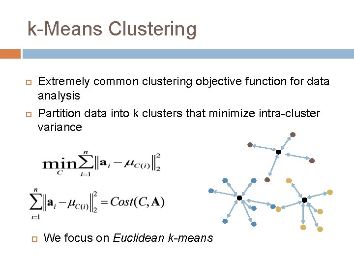
k-Means Clustering Extremely common clustering objective function for data analysis Partition data into k clusters that minimize intra-cluster variance We focus on Euclidean k-means

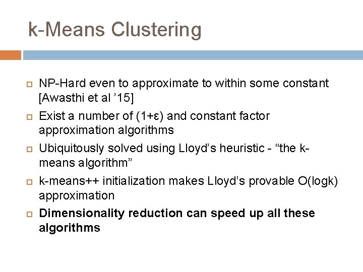
k-Means Clustering NP-Hard even to approximate to within some constant [Awasthi et al ’ 15] Exist a number of (1+ε) and constant factor approximation algorithms Ubiquitously solved using Lloyd’s heuristic - “the kmeans algorithm” k-means++ initialization makes Lloyd’s provable O(logk) approximation Dimensionality reduction can speed up all these algorithms

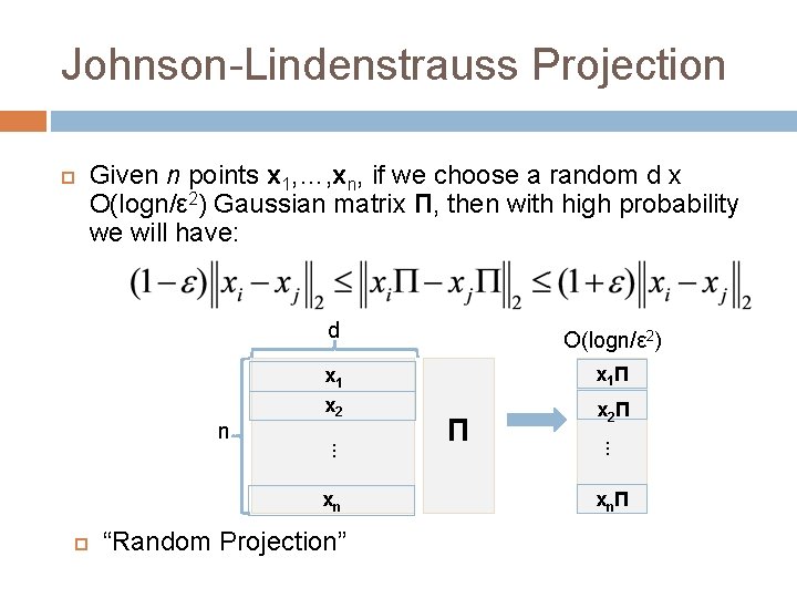
Johnson-Lindenstrauss Projection Given n points x 1, …, xn, if we choose a random d x O(logn/ε 2) Gaussian matrix Π, then with high probability we will have: O(logn/ε 2) x 1 x 2 x 1 Π xn “Random Projection” Π x 2 Π. . . n d xnΠ

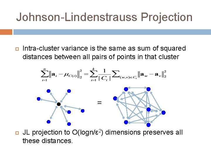
Johnson-Lindenstrauss Projection Intra-cluster variance is the same as sum of squared distances between all pairs of points in that cluster = JL projection to O(logn/ε 2) dimensions preserves all these distances.

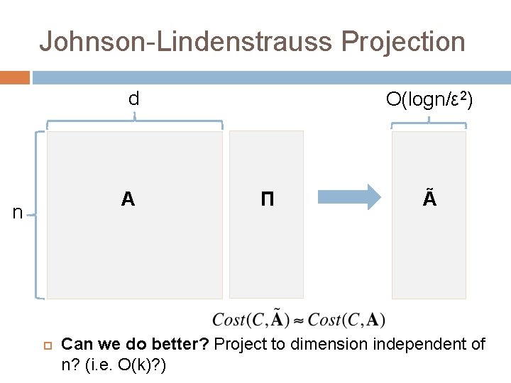
Johnson-Lindenstrauss Projection d A n O(logn/ε 2) Π Ã Can we do better? Project to dimension independent of n? (i. e. O(k)? )

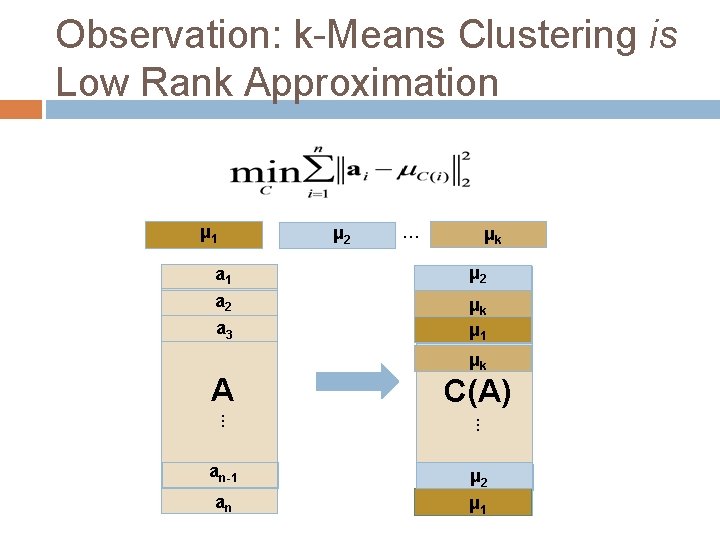
Observation: k-Means Clustering is Low Rank Approximation μ 1 μ 2 … μk a 1 μ a 21 a 2 ak 2 μ μ a 13 a 3 A μk C(A) . . . an-1 aμn-1 2 μ a 1 n an

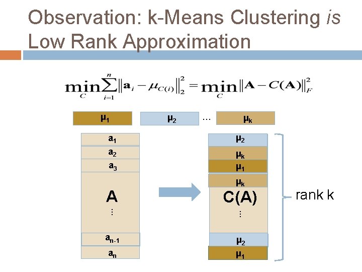
Observation: k-Means Clustering is Low Rank Approximation μ 1 μ 2 … μk a 1 μ a 21 a 2 ak 2 μ μ a 13 a 3 A μk C(A) . . . an-1 aμn-1 2 μ a 1 n an rank k

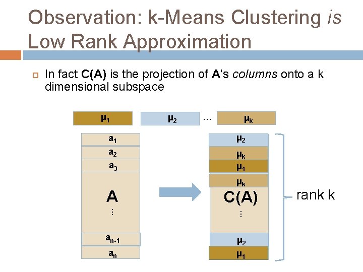
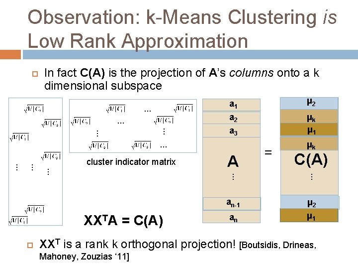
Observation: k-Means Clustering is Low Rank Approximation In fact C(A) is the projection of A’s columns onto a k dimensional subspace μ 1 μ 2 … μk a 1 μ a 21 a 2 ak 2 μ μ a 13 a 3 A μk C(A) . . . an-1 aμn-1 2 μ a 1 n an rank k

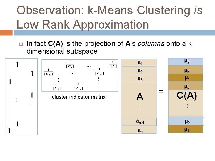
Observation: k-Means Clustering is Low Rank Approximation In fact C(A) is the projection of A’s columns onto a k dimensional subspace a 2 . . . a 3 . . . A = μ μkk C(A) . . . . cluster indicator matrix . . μ a μ 211 μ ak 2 μ a 13 a 1 . . . an-1 aμn-1 2 μ a 1 n an

Observation: k-Means Clustering is Low Rank Approximation In fact C(A) is the projection of A’s columns onto a k dimensional subspace . . . a 1 μ a 21 a 2 ak 2 μ μ μ a 131 μ 2 μk a 3 . . . XXTA = C(A) an k . . . an-1 C(A) μ. . . A. . . cluster indicator matrix = aμn-1 2 μ a 1 n XXT is a rank k orthogonal projection! [Boutsidis, Drineas, Mahoney, Zouzias ‘ 11]

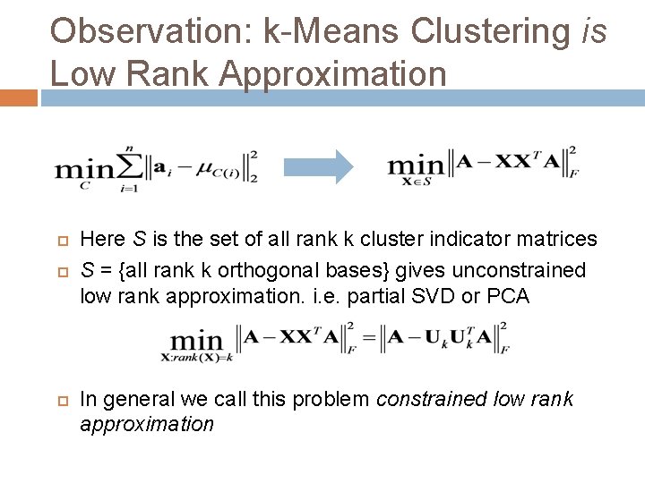
Observation: k-Means Clustering is Low Rank Approximation Here S is the set of all rank k cluster indicator matrices S = {all rank k orthogonal bases} gives unconstrained low rank approximation. i. e. partial SVD or PCA In general we call this problem constrained low rank approximation

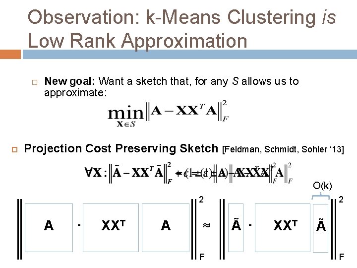
Observation: k-Means Clustering is Low Rank Approximation New goal: Want a sketch that, for any S allows us to approximate: Projection Cost Preserving Sketch [Feldman, Schmidt, Sohler ‘ 13] O(k) 2 A - XXT A ≈ F 2 Ã - XXT Ã F

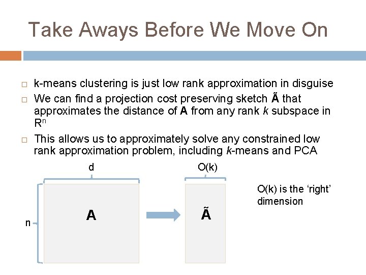
Take Aways Before We Move On k-means clustering is just low rank approximation in disguise We can find a projection cost preserving sketch à that approximates the distance of A from any rank k subspace in Rn This allows us to approximately solve any constrained low rank approximation problem, including k-means and PCA d n A O(k) à O(k) is the ‘right’ dimension

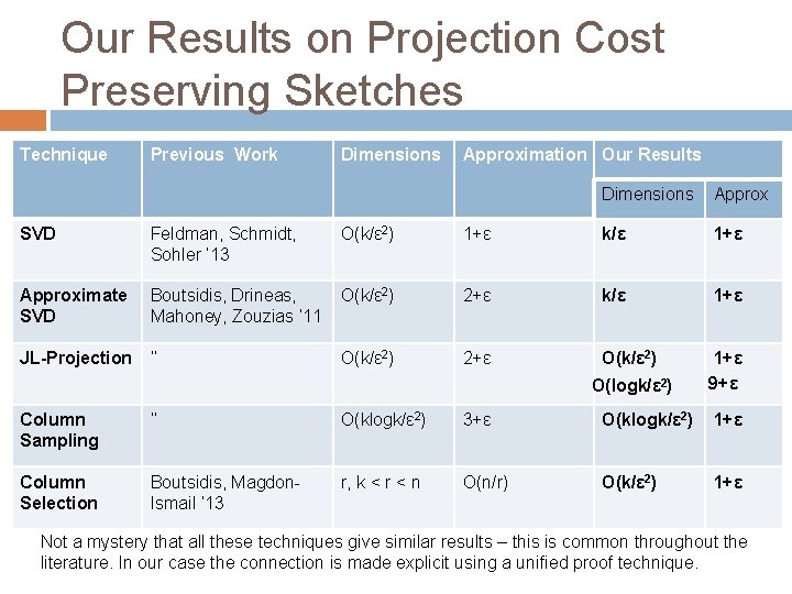
Our Results on Projection Cost Preserving Sketches Technique Previous Work Dimensions Approximation Our Results Dimensions Approx SVD Feldman, Schmidt, Sohler ‘ 13 O(k/ε 2) 1+ε k/ε 1+ε Approximate SVD Boutsidis, Drineas, Mahoney, Zouzias ‘ 11 O(k/ε 2) 2+ε k/ε 1+ε JL-Projection ‘’ O(k/ε 2) 2+ε O(k/ε 2) 1+ε 9+ε O(logk/ε 2) Column Sampling ‘’ O(klogk/ε 2) 3+ε O(klogk/ε 2) 1+ε Column Selection Boutsidis, Magdon. Ismail ‘ 13 r, k < r < n O(n/r) O(k/ε 2) 1+ε Not a mystery that all these techniques give similar results – this is common throughout the literature. In our case the connection is made explicit using a unified proof technique.

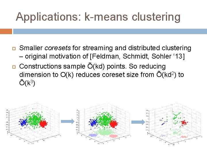
Applications: k-means clustering Smaller coresets for streaming and distributed clustering – original motivation of [Feldman, Schmidt, Sohler ‘ 13] Constructions sample Õ(kd) points. So reducing dimension to O(k) reduces coreset size from Õ(kd 2) to Õ(k 3)

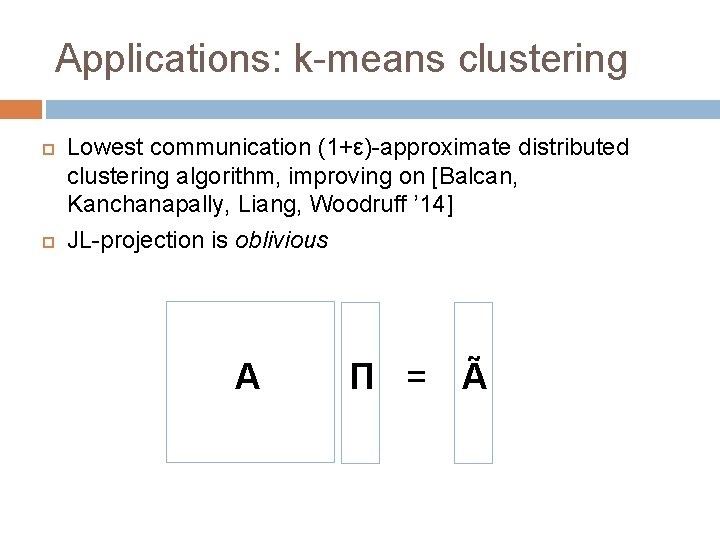
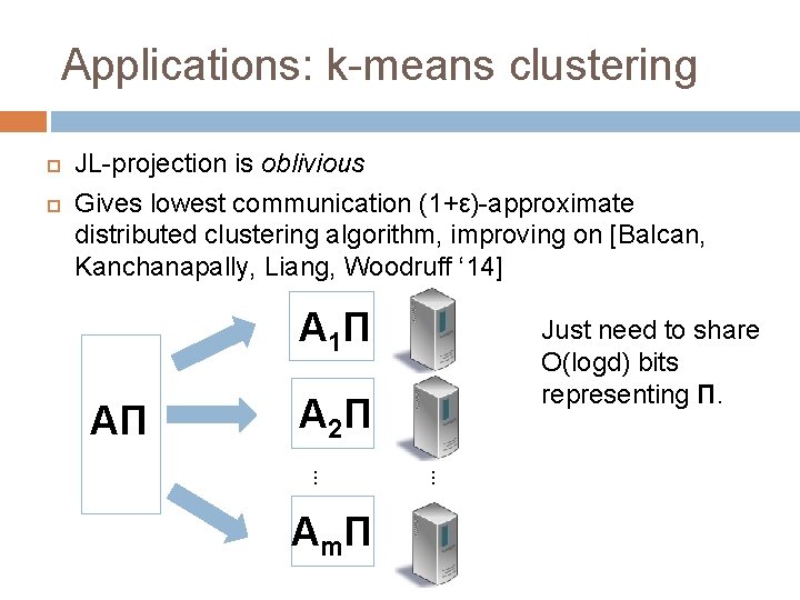
Applications: k-means clustering Lowest communication (1+ε)-approximate distributed clustering algorithm, improving on [Balcan, Kanchanapally, Liang, Woodruff ’ 14] JL-projection is oblivious A Π = Ã

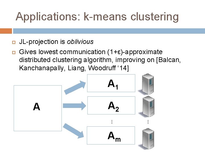
Applications: k-means clustering JL-projection is oblivious Gives lowest communication (1+ε)-approximate distributed clustering algorithm, improving on [Balcan, Kanchanapally, Liang, Woodruff ‘ 14] A 1 A A 2. . . Am

Applications: k-means clustering JL-projection is oblivious Gives lowest communication (1+ε)-approximate distributed clustering algorithm, improving on [Balcan, Kanchanapally, Liang, Woodruff ‘ 14] A 1Π AΠ Just need to share O(logd) bits representing Π. A 2Π. . . A mΠ

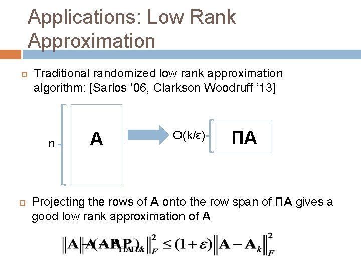
Applications: Low Rank Approximation Traditional randomized low rank approximation algorithm: [Sarlos ’ 06, Clarkson Woodruff ‘ 13] n A O(k/ε) ΠA Projecting the rows of A onto the row span of ΠA gives a good low rank approximation of A

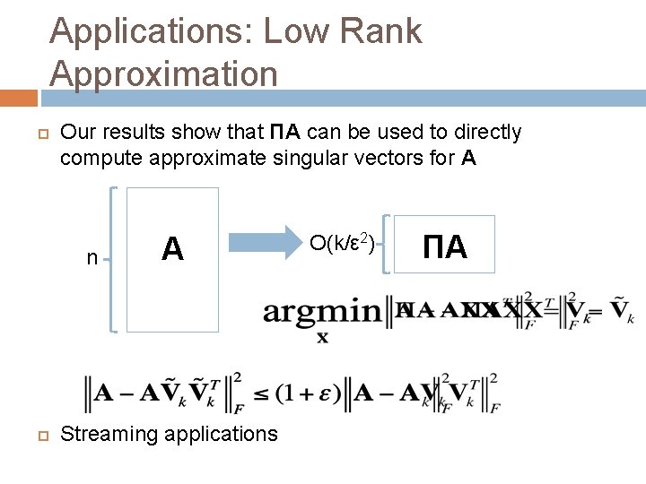
Applications: Low Rank Approximation Our results show that ΠA can be used to directly compute approximate singular vectors for A n A Streaming applications O(k/ε 2) ΠA

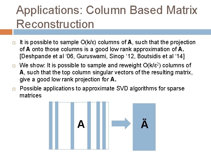
Applications: Column Based Matrix Reconstruction It is possible to sample O(k/ε) columns of A, such that the projection of A onto those columns is a good low rank approximation of A. [Deshpande et al ‘ 06, Guruswami, Sinop ‘ 12, Boutsidis et al ‘ 14] We show: It is possible to sample and reweight O(k/ε 2) columns of A, such that the top column singular vectors of the resulting matrix, give a good low rank projection for A. Possible applications to approximate SVD algorithms for sparse matrices A Ã

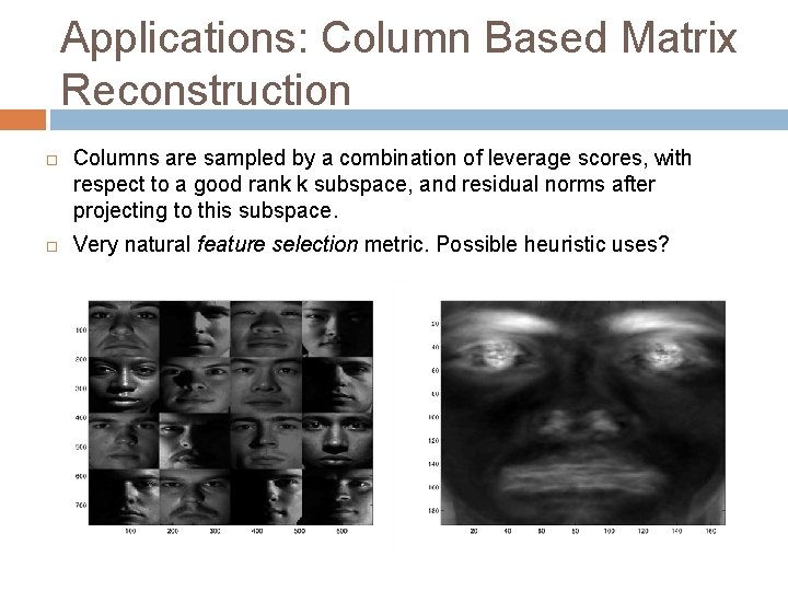
Applications: Column Based Matrix Reconstruction Columns are sampled by a combination of leverage scores, with respect to a good rank k subspace, and residual norms after projecting to this subspace. Very natural feature selection metric. Possible heuristic uses?

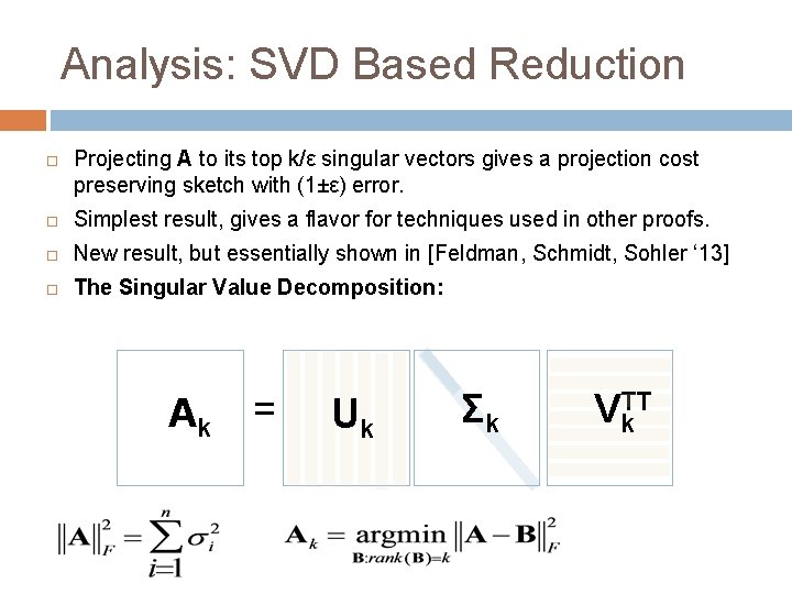
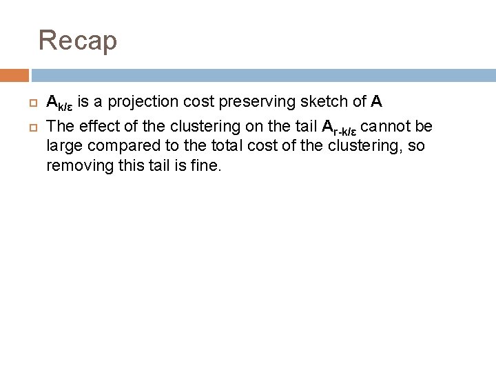
Analysis: SVD Based Reduction Projecting A to its top k/ε singular vectors gives a projection cost preserving sketch with (1±ε) error. Simplest result, gives a flavor for techniques used in other proofs. New result, but essentially shown in [Feldman, Schmidt, Sohler ‘ 13] The Singular Value Decomposition: Ak = Uk Σk VTk. T

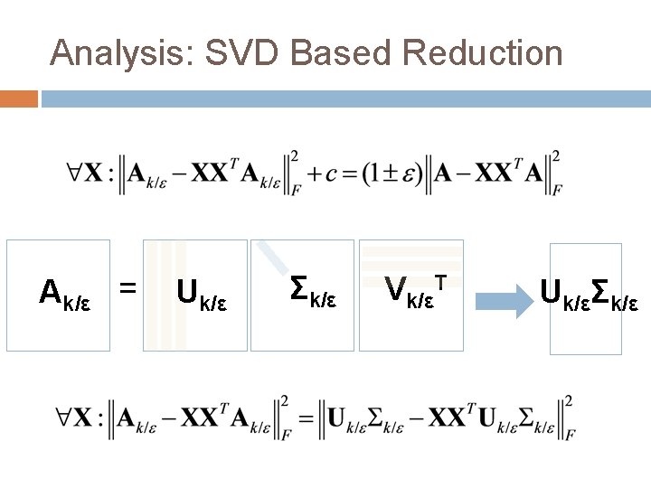
Analysis: SVD Based Reduction Ak/ε = Uk/ε Σk/ε Vk/εT Uk/εΣk/ε

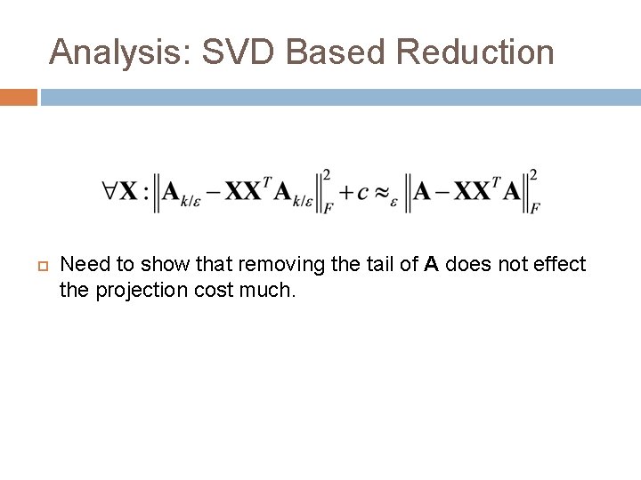
Analysis: SVD Based Reduction Need to show that removing the tail of A does not effect the projection cost much.

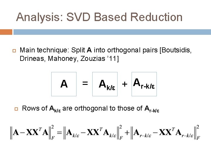
Analysis: SVD Based Reduction Main technique: Split A into orthogonal pairs [Boutsidis, Drineas, Mahoney, Zouzias ’ 11] A = Ak/ε + Ar-k/ε Rows of Ak/ε are orthogonal to those of Ar-k/ε

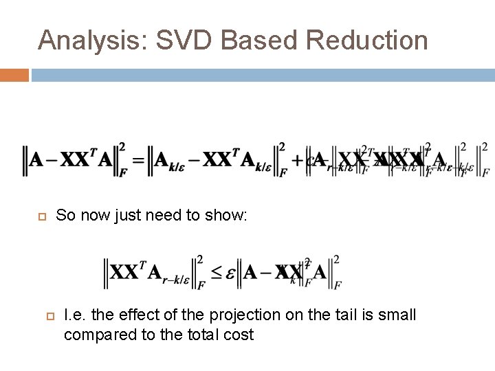
Analysis: SVD Based Reduction So now just need to show: I. e. the effect of the projection on the tail is small compared to the total cost

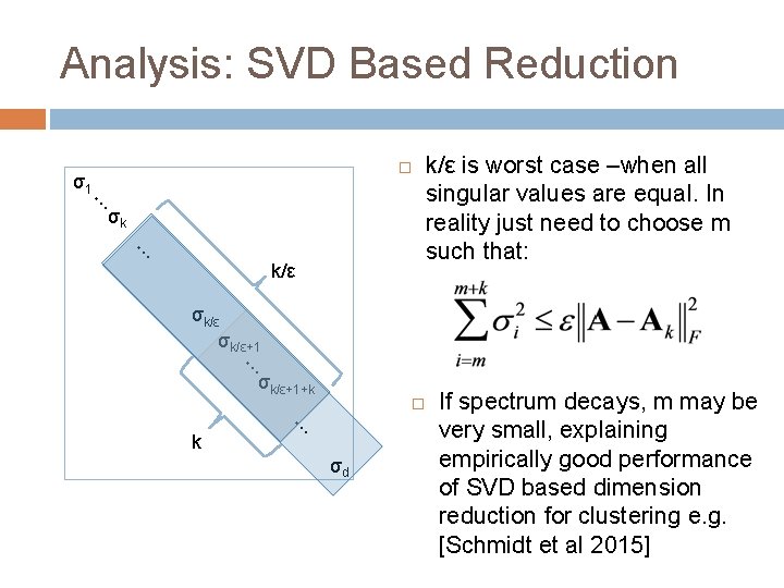
Analysis: SVD Based Reduction σ1 … σk … k/ε σk/ε+1 … σk/ε+1+k … k σd

Analysis: SVD Based Reduction σ1 … σk … k/ε is worst case –when all singular values are equal. In reality just need to choose m such that: σk/ε+1 … σk/ε+1+k … k σd If spectrum decays, m may be very small, explaining empirically good performance of SVD based dimension reduction for clustering e. g. [Schmidt et al 2015]

Analysis: SVD Based Reduction SVD based dimension reduction is very popular in practice with m = k This is because computing the top k singular vectors is viewed as a continuous relaxation of k-means clustering Our analysis gives a better understanding of the connection between SVD/PCA and k-means clustering.

Recap Ak/ε is a projection cost preserving sketch of A The effect of the clustering on the tail Ar-k/ε cannot be large compared to the total cost of the clustering, so removing this tail is fine.

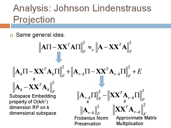
Analysis: Johnson Lindenstrauss Projection Same general idea. ≈ Frobenius Norm Preservation ≈ ≈ Subspace Embedding property of O(k/ε 2) dimension RP on k dimensional subspace Approximate Matrix Multiplication

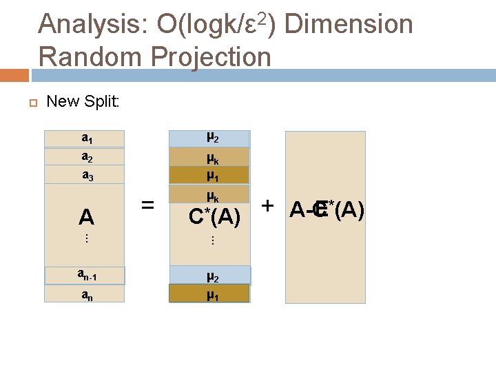
Analysis: O(logk/ε 2) Dimension Random Projection New Split: a 1 μ a 21 a 2 ak 2 μ μ a 13 a 3 A = μk C*(A) . . . an-1 aμn-1 2 μ a 1 n an + A-C E*(A)

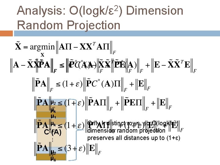
Analysis: O(logk/ε 2) Dimension Random Projection μ a 21 ak 2 μ μ a 13 μk C*(A). . . aμn-2 1μ a 1 n Only k distinct rows, so O(logk/ε 2) dimension random projection preserves all distances up to (1+ε)

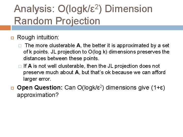
Analysis: O(logk/ε 2) Dimension Random Projection Rough intuition: � � The more clusterable A, the better it is approximated by a set of k points. JL projection to O(log k) dimensions preserves the distances between these points. If A is not well clusterable, then the JL projection does not preserve much about A, but that’s ok because we can afford larger error. Open Question: Can O(logk/ε 2) dimensions give (1+ε) approximation?

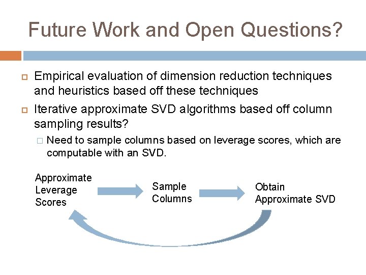
Future Work and Open Questions? Empirical evaluation of dimension reduction techniques and heuristics based off these techniques Iterative approximate SVD algorithms based off column sampling results? � Need to sample columns based on leverage scores, which are computable with an SVD. Approximate Leverage Scores Sample Columns Obtain Approximate SVD