Dimensionality Reduction A Comparative Study AAYUSH MUDGAL 12008

Dimensionality Reduction : A Comparative Study AAYUSH MUDGAL [12008] SHEALLIKA SINGH [12665]

What is Dimensionality Reduction ? Mapping of data to lower dimension such that: • uninformative variance is discarded, • or a subspace where data lives is detected Why dimensionality reduction ? • • Reduce Curse of dimensionality: Requires larger number of observations to train the model efficiently Better interpretation of models and visualization of data Reduces the computational cost

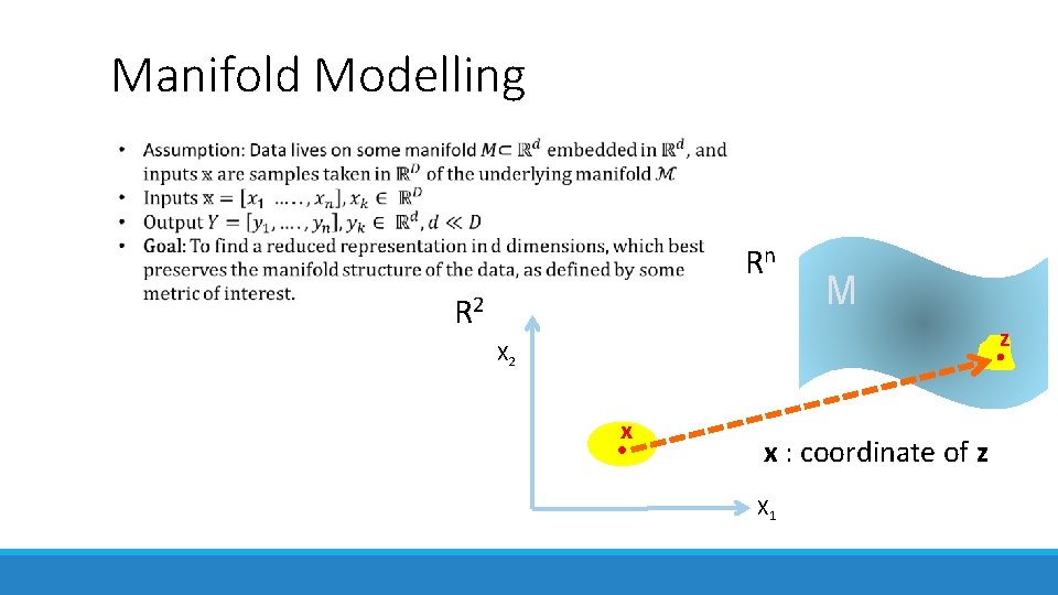
Assumptions of dimensionality reduction Higher dimensional Data lies on a much lower dimensional manifold

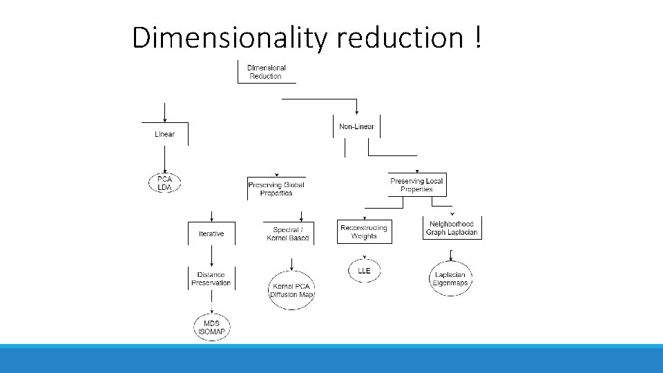
Dimensionality reduction !

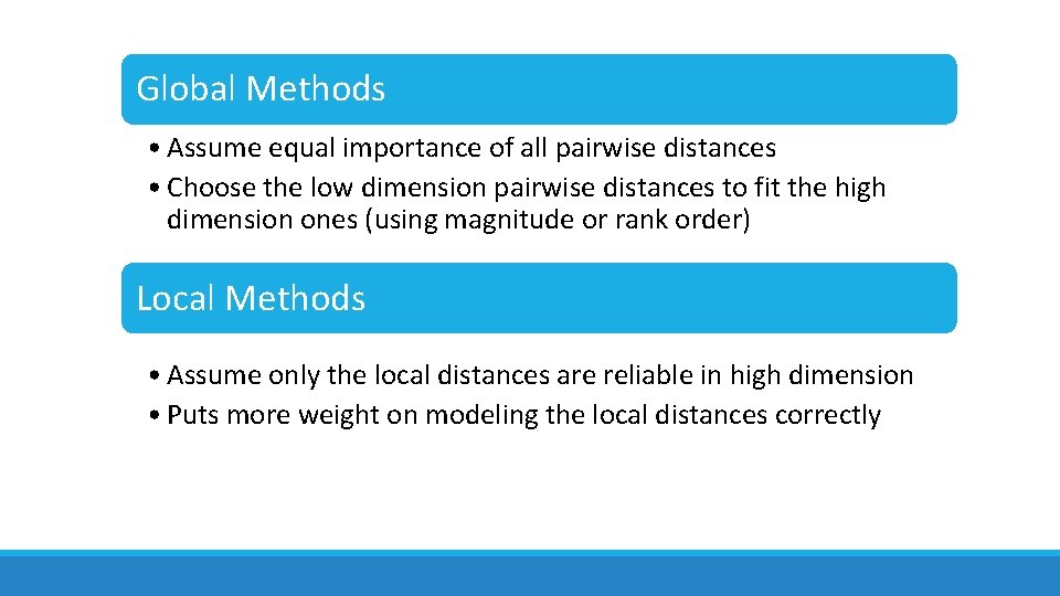
Global Methods • Assume equal importance of all pairwise distances • Choose the low dimension pairwise distances to fit the high dimension ones (using magnitude or rank order) Local Methods • Assume only the local distances are reliable in high dimension • Puts more weight on modeling the local distances correctly

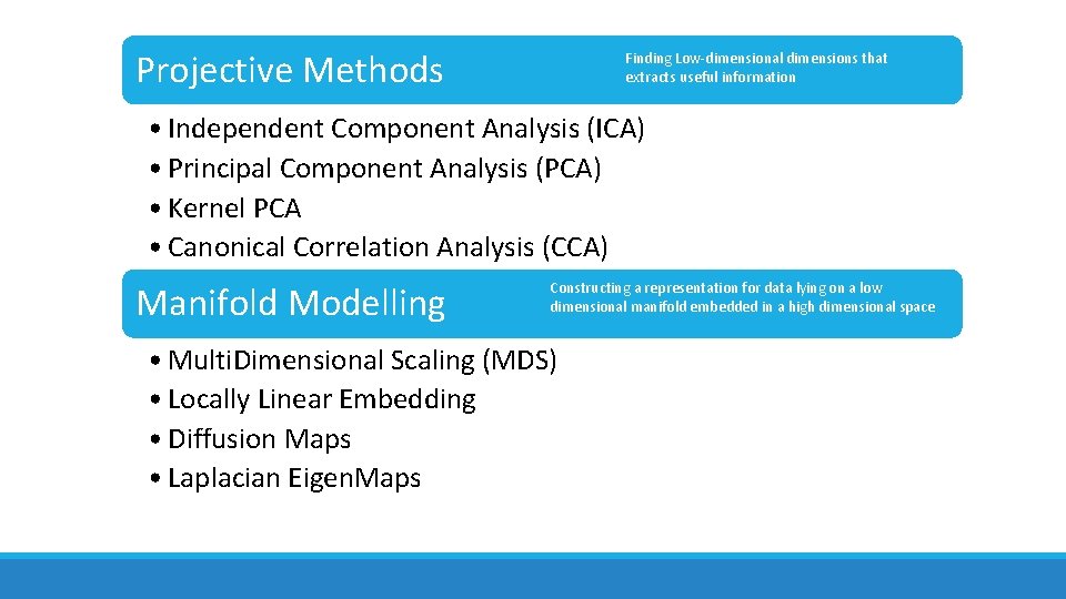
Projective Methods Finding Low-dimensional dimensions that extracts useful information • Independent Component Analysis (ICA) • Principal Component Analysis (PCA) • Kernel PCA • Canonical Correlation Analysis (CCA) Manifold Modelling Constructing a representation for data lying on a low dimensional manifold embedded in a high dimensional space • Multi. Dimensional Scaling (MDS) • Locally Linear Embedding • Diffusion Maps • Laplacian Eigen. Maps

Independent Component Analysis • • Motivation for ICA: Cocktail party problem Separate the mixed signal into sources Assumption: different sources are independent To give non trivial results source signals are required to be non-Gaussian

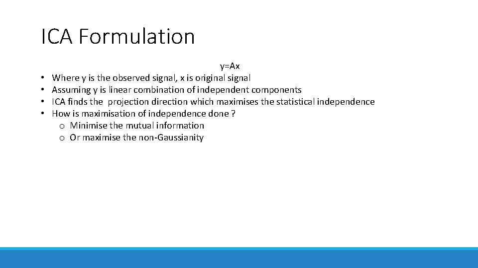
ICA Formulation • • y=Ax Where y is the observed signal, x is original signal Assuming y is linear combination of independent components ICA finds the projection direction which maximises the statistical independence How is maximisation of independence done ? o Minimise the mutual information o Or maximise the non-Gaussianity

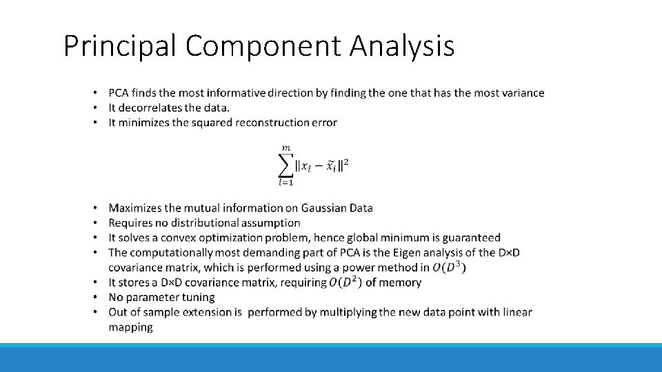
Principal Component Analysis

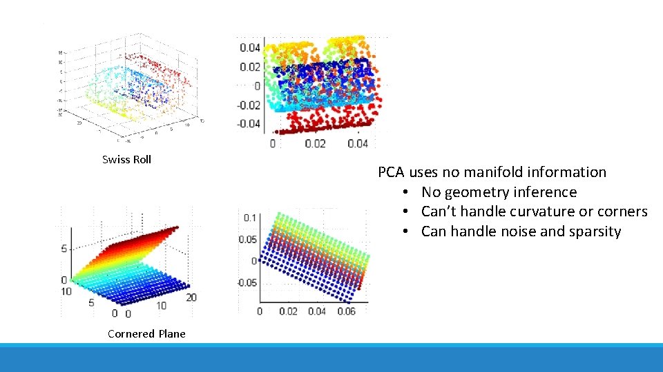
Swiss Roll Cornered Plane PCA uses no manifold information • No geometry inference • Can’t handle curvature or corners • Can handle noise and sparsity

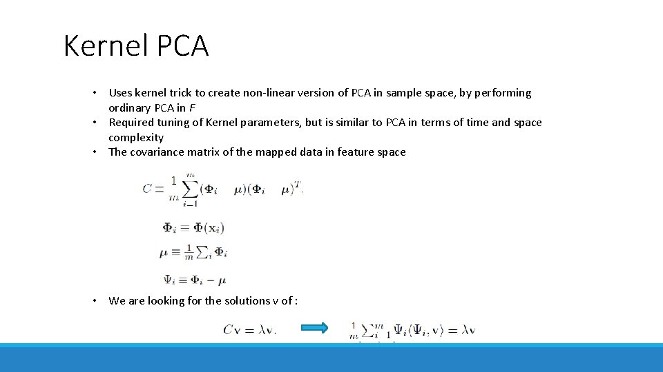
Kernel PCA • Uses kernel trick to create non-linear version of PCA in sample space, by performing ordinary PCA in F • Required tuning of Kernel parameters, but is similar to PCA in terms of time and space complexity • The covariance matrix of the mapped data in feature space • We are looking for the solutions v of :

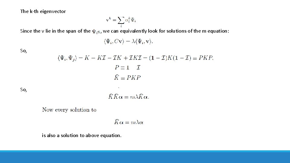
The k-th eigenvector Since the v lie in the span of the , we can equivalently look for solutions of the m equation: So, ` is also a solution to above equation.

Algorithm : Kernel PCA (schematic)

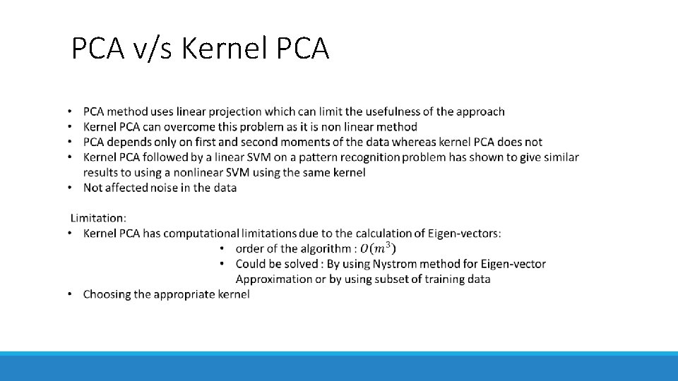
PCA v/s Kernel PCA

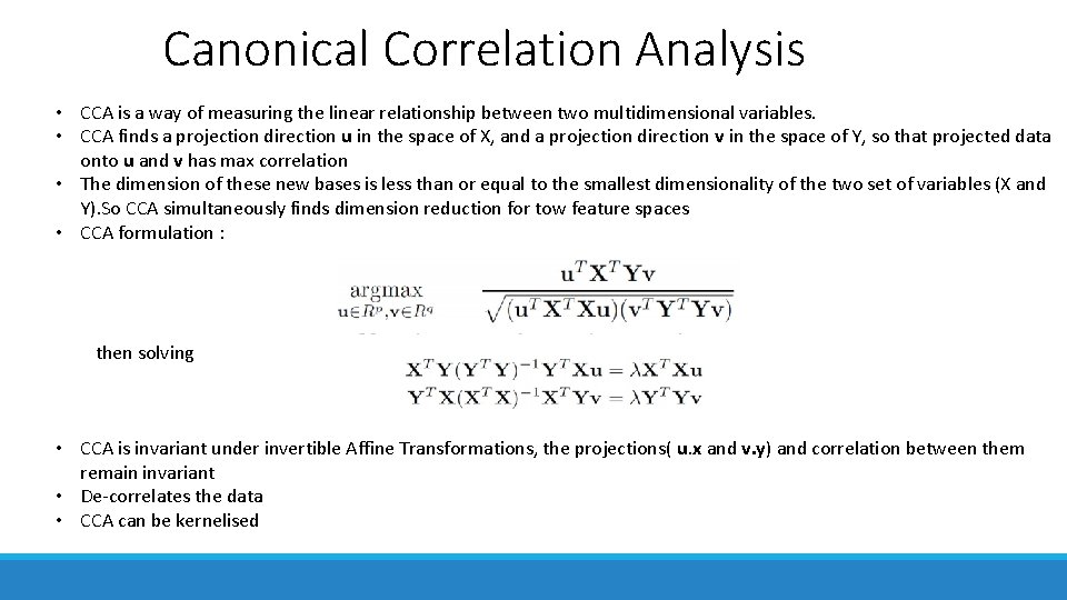
Canonical Correlation Analysis • CCA is a way of measuring the linear relationship between two multidimensional variables. • CCA finds a projection direction u in the space of X, and a projection direction v in the space of Y, so that projected data onto u and v has max correlation • The dimension of these new bases is less than or equal to the smallest dimensionality of the two set of variables (X and Y). So CCA simultaneously finds dimension reduction for tow feature spaces • CCA formulation : then solving • CCA is invariant under invertible Affine Transformations, the projections( u. x and v. y) and correlation between them remain invariant • De-correlates the data • CCA can be kernelised

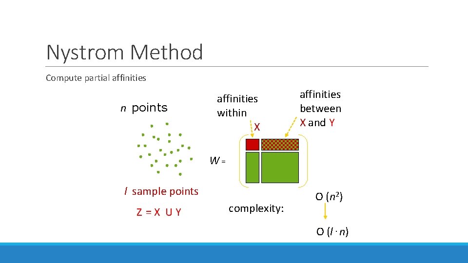
Nystrom Method Compute partial affinities n points affinities within X affinities between X and Y W = l sample points Z = X U Y complexity: O (n 2) O (l. n)

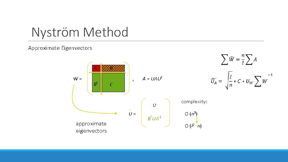
Nyström Method Approximate Eigenvectors A W = BT B C U U = approximate eigenvectors , A = UΛUT BTUΛ-1 complexity: O (n 3) O (l 2. n)

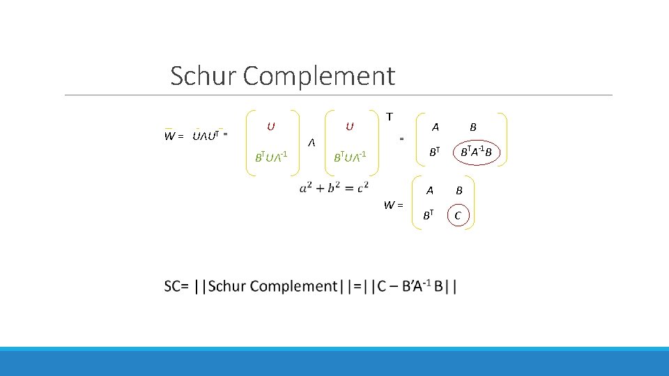
Schur Complement U W = UΛUT = T B UΛ Λ -1 T U = T B UΛ -1 W = A B BT BTA-1 B A B BT C

Manifold Modelling Rn R 2 M z X 2 x x : coordinate of z X 1

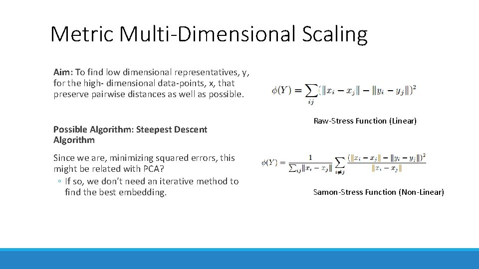
Metric Multi-Dimensional Scaling Aim: To find low dimensional representatives, y, for the high- dimensional data-points, x, that preserve pairwise distances as well as possible. Possible Algorithm: Steepest Descent Algorithm Since we are, minimizing squared errors, this might be related with PCA? ◦ If so, we don’t need an iterative method to find the best embedding. Raw-Stress Function (Linear) Samon-Stress Function (Non-Linear)

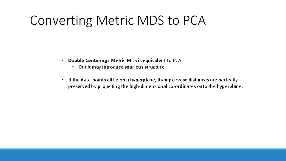
Converting Metric MDS to PCA • Double Centering : Metric MDS is equivalent to PCA • But it may introduce spurious structure • If the data-points all lie on a hyperplane, their pairwise distances are perfectly preserved by projecting the high-dimensional co-ordinates onto the hyperplane.

Multi-Dimensional Scaling : Summary • MDS could be extended for use on ordinal values • Landmark MDS : It is used to solve the bottleneck in classical MDS, and uses a subset of data. Scalability is increased but approximation is noise sensitive • If the data-points all lie on a hyperplane, their pairwise distances are perfectly preserved by projecting the high-dimensional co-ordinates onto the hyperplane • Like PCA it can neither understand geometry nor handle non-convexity, and curvature • Does not require assumptions of linearity, metricity, or multivariate normality

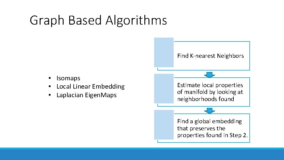
Graph Based Algorithms Find K-nearest Neighbors • Isomaps • Local Linear Embedding • Laplacian Eigen. Maps Estimate local properties of manifold by looking at neighborhoods found Find a global embedding that preserves the properties found in Step 2.

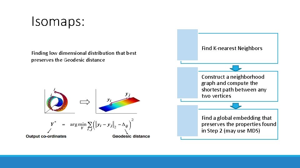
Isomaps: Finding low dimensional distribution that best preserves the Geodesic distance Find K-nearest Neighbors Construct a neighborhood graph and compute the shortest path between any two vertices Find a global embedding that preserves the properties found in Step 2 (may use MDS)

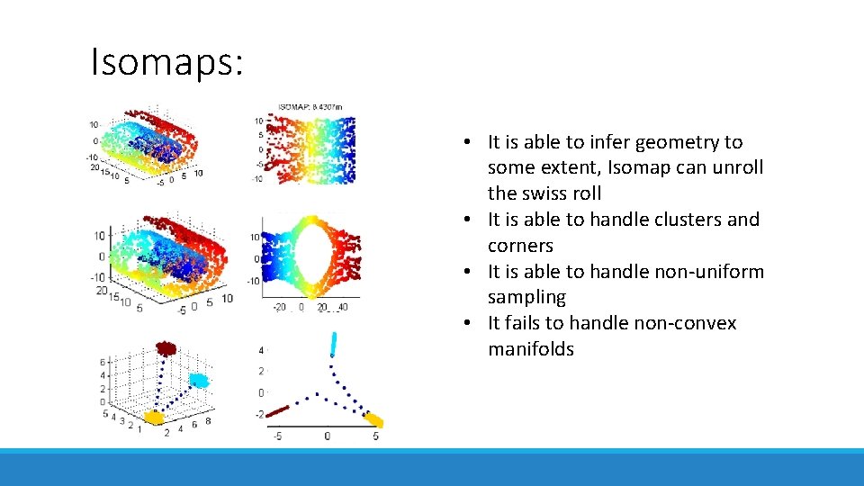
Isomaps: • It is able to infer geometry to some extent, Isomap can unroll the swiss roll • It is able to handle clusters and corners • It is able to handle non-uniform sampling • It fails to handle non-convex manifolds

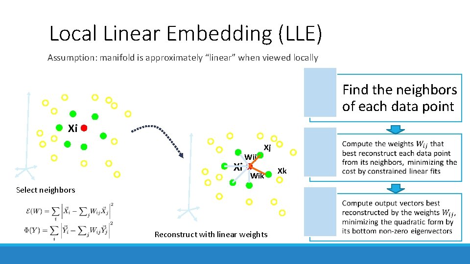
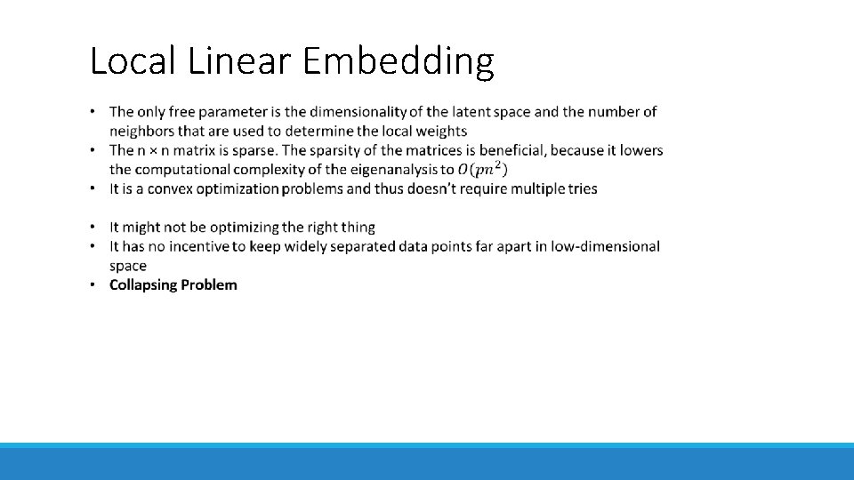
Local Linear Embedding (LLE) Assumption: manifold is approximately “linear” when viewed locally Find the neighbors of each data point Xi Xi Wij Xj Wik Xk Select neighbors Reconstruct with linear weights 26

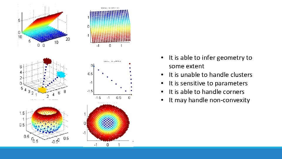
• It is able to infer geometry to some extent • It is unable to handle clusters • It is sensitive to parameters • It is able to handle corners • It may handle non-convexity

Local Linear Embedding

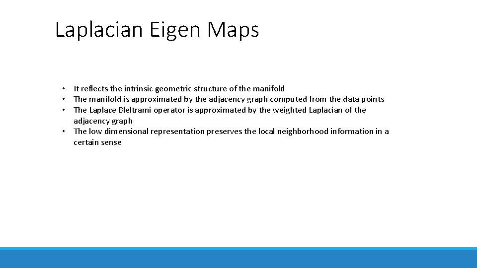
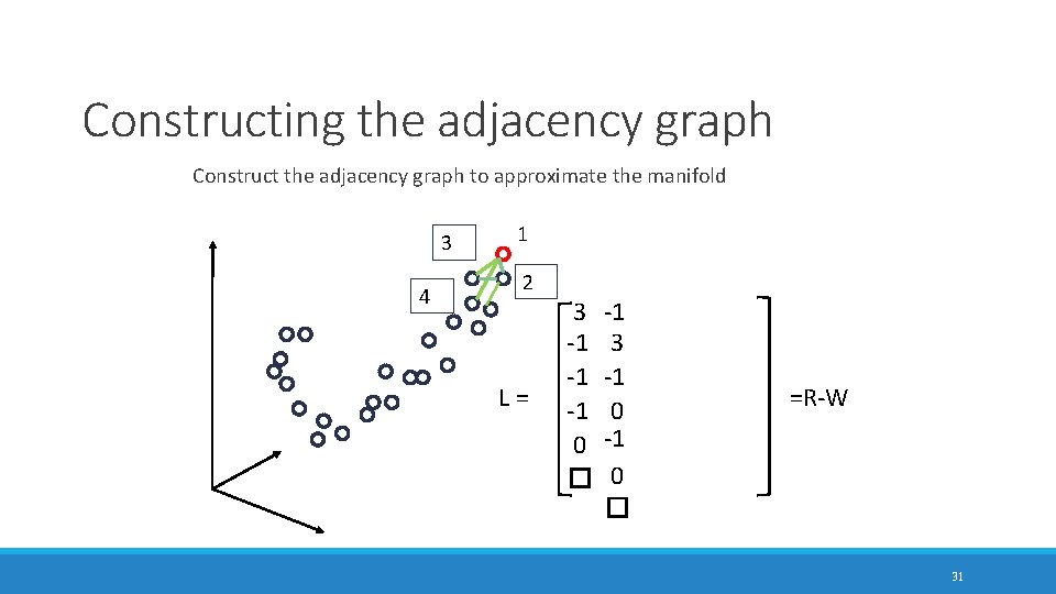
Laplacian Eigen Maps • It reflects the intrinsic geometric structure of the manifold • The manifold is approximated by the adjacency graph computed from the data points • The Laplace Bleltrami operator is approximated by the weighted Laplacian of the adjacency graph • The low dimensional representation preserves the local neighborhood information in a certain sense

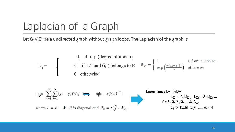
Laplacian of a Graph Let G(V, E) be a undirected graph without graph loops. The Laplacian of the graph is dij if i=j (degree of node i) Lij = -1 if i≠j and (i, j) belongs to E 0 otherwise Eigenmaps Ly = λDy Ly 0 = λ 0 Dy 0, Ly 1 = λ 1 Dy 1 … 0= λ 0≦ λ 1≦… ≦ λn-1 xi (y 0(i), y 1(i), …, ym(i)) 30

Constructing the adjacency graph Construct the adjacency graph to approximate the manifold 3 4 1 2 L = 3 -1 -1 -1 0 � -1 3 -1 0 � =R-W 31

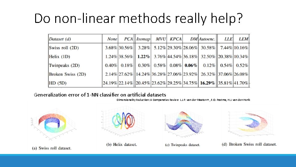
Do non-linear methods really help? Generalization error of 1 -NN classifier on artificial datasets Dimensionality Reduction: A Comparative Review L. J. P. van der Maaten ∗ , E. O. Postma, H. J. van den Herik

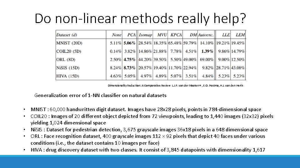
Do non-linear methods really help? Dimensionality Reduction: A Comparative Review L. J. P. van der Maaten ∗ , E. O. Postma, H. J. van den Herik Generalization error of 1 -NN classifier on natural datasets • MNIST : 60, 000 handwritten digit dataset. Images have 28 x 28 pixels, points in 784 -dimensional space • COIL 20 : Images of 20 different object depicted from 72 viewpoints, leading to 1, 440 images (32 x 32) pixels yielding 1, 024 dimensional space • Ni. SIS : Dataset for pedestrian detection, 3, 675 grayscale images 36 x 18 pixels in a 648 dimensional space • ORL : Face recognition dataset, 400 grayscale images 112 × 92 pixels that depict 40 faces under various conditions (i. e. , the dataset contains 10 images per face) • HIVA : drug discovery dataset with two classes. It consist of 3, 845 datapoints with dimensionality 1, 617

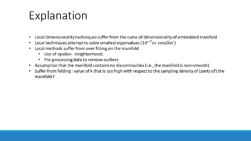
Explanation

Conclusion • Nonlinear techniques do not yet clearly outperform traditional PCA • On selected datasets, nonlinear techniques outperform linear techniques, but on perform poorly oon various other natural datasets • Need to shift focus towards development of techniques that have objective functions that can be optimized well in practice. • Strong performance of autoencoders reveal that these objective functions may not be necessarily convex

Conclusion • Laplacian eigenmap provides a computationally efficient approach to non-linear dimensionality reduction that has locality preserving properties • Ham et al. [46] show that Laplacian eigenmaps, LLE, and Isomap can be viewed as variants of kernel PCA. • Platt [70] links several flavors of MDS by showing how landmark MDS is in fact Nystr¨om algorithms • Despite the mathematical similarities of LLE, Isomap, and Laplacian Eigenmaps, their different geometrical roots result in different properties: • for example, for data which lies on a manifold of dimension d embedded in a higher dimensional space, the eigenvalue spectrum of the LLE and Laplacian Eigenmaps algorithms do not reveal anything about d, whereas the spectrum for Isomap (and MDS) does.

References • Dimensionality Reduction: A Comparative Review L. J. P. van der Maaten ∗ , E. O. Postma, H. J. van den Herik • Large-Scale Manifold Learning, Ameet Talwalkar and Sanjiv Kumar and Henry A. Rowley, Computer Vision and Pattern Recognition (CVPR), 2008 • Laplacian Eigenmaps for Dimensionality Reduction and Data Representation, M. Belkin and P. Niyogi, Neural Computation, pp. 1373– 1396, 2003 • Dimensionality Reduction: A Guided Tour, C. J. C. Burges, Foundations and Trends in Machine Learning, 2010 • An Introduction to Locally Linear Embedding, Lawrence K. Saul, AT&T Labs – Research, 180 Park Ave, Florham Park, NJ 07932 USA • Lecture Notes on Data Mining by Cosma Shalizi, http: //www. stat. cmu. edu/~cshalizi/350/ • Probabilistic Principal Component Analysis, Journal of the Royal Statistical Society, Seires B, 61 Part 3