Dimension reduction PCA and Clustering Agnieszka S Juncker

Dimension reduction : PCA and Clustering Agnieszka S. Juncker Slides: Christopher Workman and Agnieszka S. Juncker Center for Biological Sequence Analysis DTU

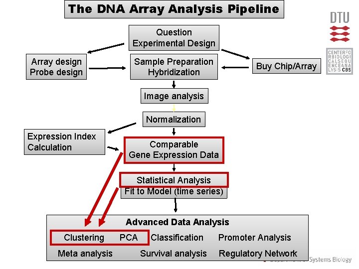
The DNA Array Analysis Pipeline Question Experimental Design Array design Probe design Sample Preparation Hybridization Buy Chip/Array Image analysis Normalization Expression Index Calculation Comparable Gene Expression Data Statistical Analysis Fit to Model (time series) Advanced Data Analysis Clustering Meta analysis PCA Classification Survival analysis Promoter Analysis Regulatory Network

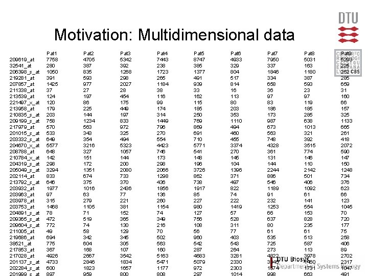
Motivation: Multidimensional data 209619_at 32541_at 206398_s_at 219281_at 207857_at 211338_at 213539_at 221497_x_at 213958_at 210835_s_at 209199_s_at 217979_at 201015_s_at 203332_s_at 204670_x_at 208788_at 210784_x_at 204319_s_at 205049_s_at 202114_at 213792_s_at 203932_at 203963_at 203978_at 203753_at 204891_s_at 209365_s_at 209604_s_at 211005_at 219686_at 38521_at 217853_at 217028_at 201137_s_at 202284_s_at Pat 1 7758 280 1050 391 1425 37 124 120 179 203 758 570 533 649 5577 648 142 298 3294 833 646 1977 97 315 1468 78 472 772 49 694 775 367 4926 4733 600 Pat 2 4705 387 835 593 977 27 197 86 225 144 1234 563 343 354 3216 327 151 172 1351 674 375 1016 63 279 1105 71 519 74 58 342 604 168 2667 2846 1823 Pat 3 5342 392 1268 298 2027 28 454 175 449 197 833 972 325 494 5323 1057 144 200 2080 733 370 2436 77 221 381 152 365 130 129 345 305 107 3542 1834 1657 Pat 4 7443 238 1723 265 1184 38 116 99 174 314 1449 796 270 554 4423 746 173 298 2066 1298 436 1856 136 260 1154 74 349 216 70 502 563 160 5163 5471 1177 Pat 5 8747 385 1377 491 939 33 162 115 185 250 769 869 691 710 5771 541 148 196 3726 862 738 1917 85 227 980 127 756 108 56 960 542 287 4683 5079 972 Pat 6 4933 329 804 517 814 16 113 80 203 353 1110 494 460 455 3374 270 145 104 1396 371 497 822 74 222 1419 57 528 311 77 403 543 264 3281 2330 2303 Pat 7 7950 337 1846 334 658 36 97 83 186 173 987 673 563 748 4328 361 131 144 2244 886 546 1189 91 232 1253 66 637 80 61 535 725 273 4822 3345 1574 Pat 8 5031 163 1180 387 593 23 97 119 185 285 638 1013 321 392 3515 774 146 110 2142 501 406 1092 61 141 554 153 828 235 61 513 587 113 3978 1460 1731 Pat 9 5293 225 252 285 659 31 160 66 157 325 1133 665 261 418 2072 590 147 150 1248 734 376 623 66 123 1045 70 720 177 75 258 406 89 2702 2317 1047

PCA

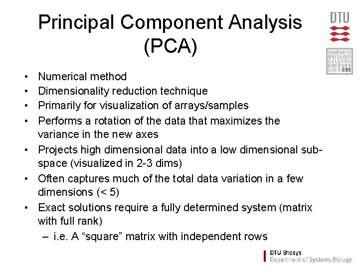
Principal Component Analysis (PCA) • • Numerical method Dimensionality reduction technique Primarily for visualization of arrays/samples Performs a rotation of the data that maximizes the variance in the new axes • Projects high dimensional data into a low dimensional subspace (visualized in 2 -3 dims) • Often captures much of the total data variation in a few dimensions (< 5) • Exact solutions require a fully determined system (matrix with full rank) – i. e. A “square” matrix with independent rows

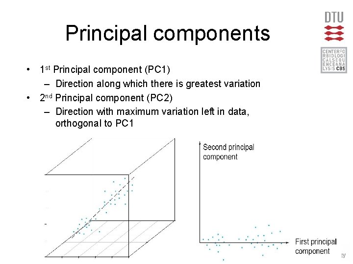
Principal components • 1 st Principal component (PC 1) – Direction along which there is greatest variation • 2 nd Principal component (PC 2) – Direction with maximum variation left in data, orthogonal to PC 1

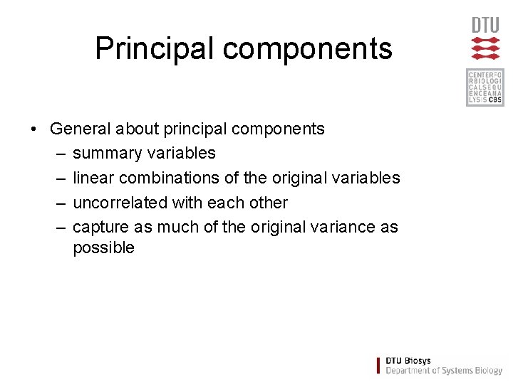
Principal components • General about principal components – summary variables – linear combinations of the original variables – uncorrelated with each other – capture as much of the original variance as possible

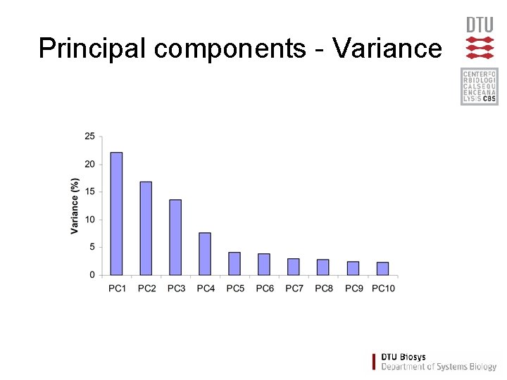
Principal components - Variance

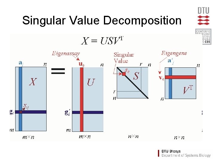
Singular Value Decomposition

Singular Value Decomposition • Requirements: – No missing values – “Centered” observations, i. e. normalize data such that each gene has mean = 0

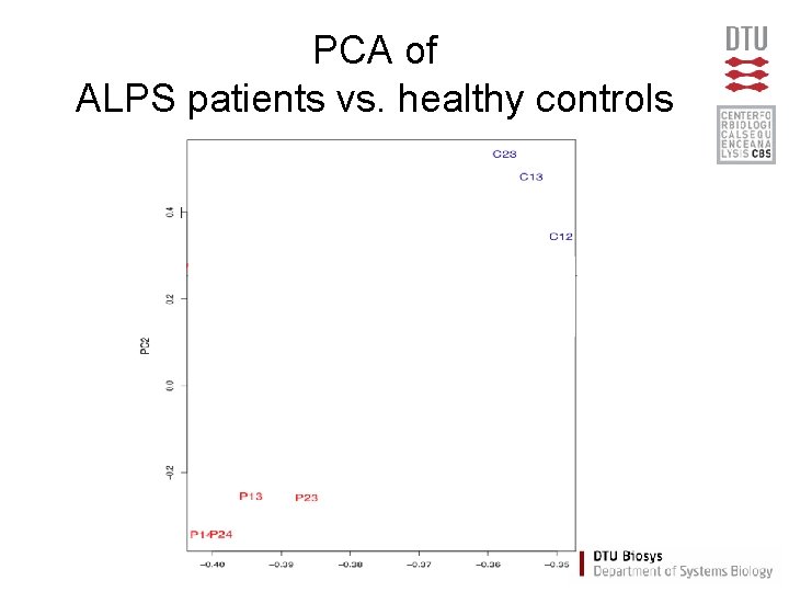
PCA of ALPS patients vs. healthy controls

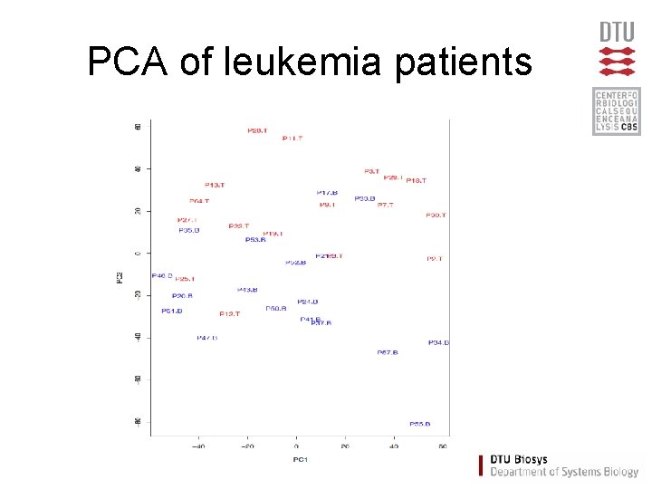
PCA of leukemia patients

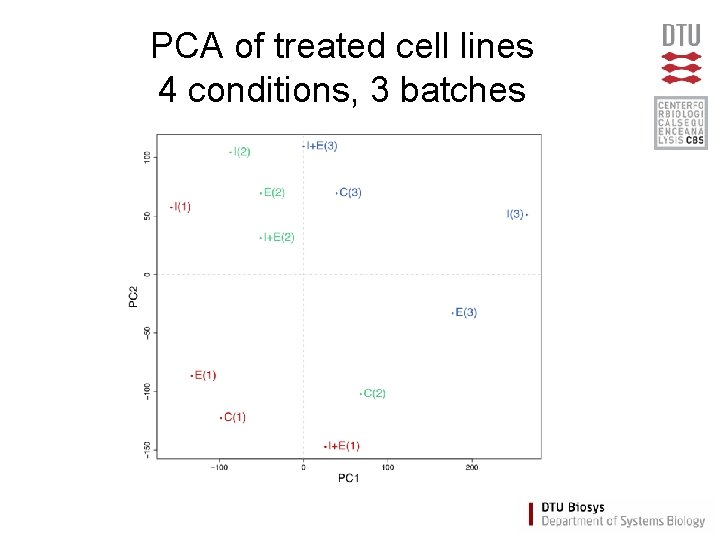
PCA of treated cell lines 4 conditions, 3 batches

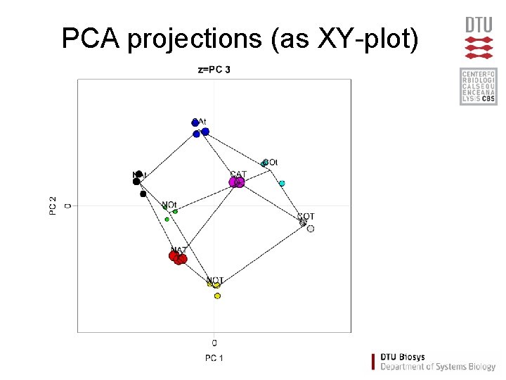
PCA projections (as XY-plot)

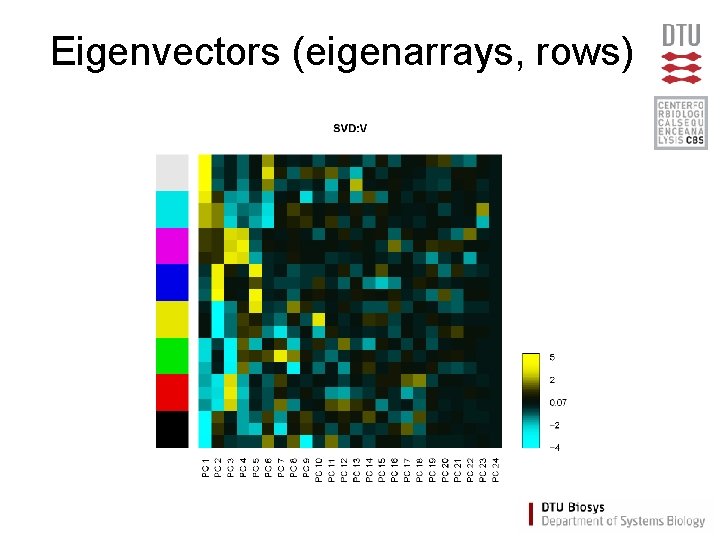
Eigenvectors (eigenarrays, rows)

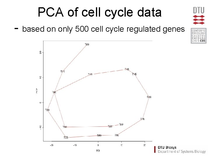
PCA of cell cycle data - based on only 500 cell cycle regulated genes

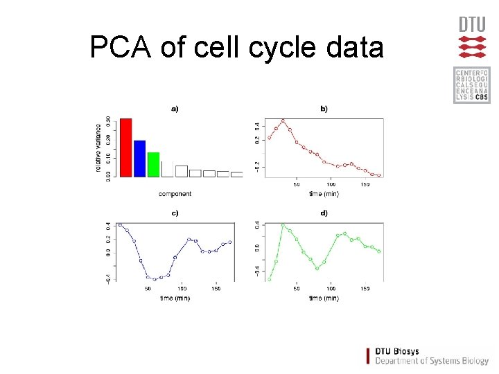
PCA of cell cycle data

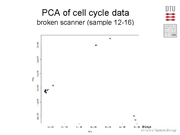
PCA of cell cycle data broken scanner (sample 12 -16)

Clustering

Why do we cluster? • Organize observed data into meaningful structures • Summarize large data sets • Used when we have no a priori hypotheses

Many types of clustering methods • Method: – K-class – Hierarchical, e. g. UPGMA • Agglomerative (bottom-up) • Divisive (top-down) – Graph theoretic

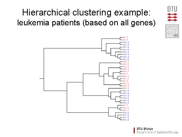
Hierarchical clustering • Representation of all pair-wise distances • Parameters: none (distance measure) • Results: – One large cluster – Hierarchical tree (dendrogram) • Deterministic

Hierarchical clustering – UPGMA Algorithm • Assign each item to its own cluster • Join the nearest clusters • Re-estimate the distance between clusters • Repeat for 1 to n

Hierarchical clustering

Hierarchical clustering

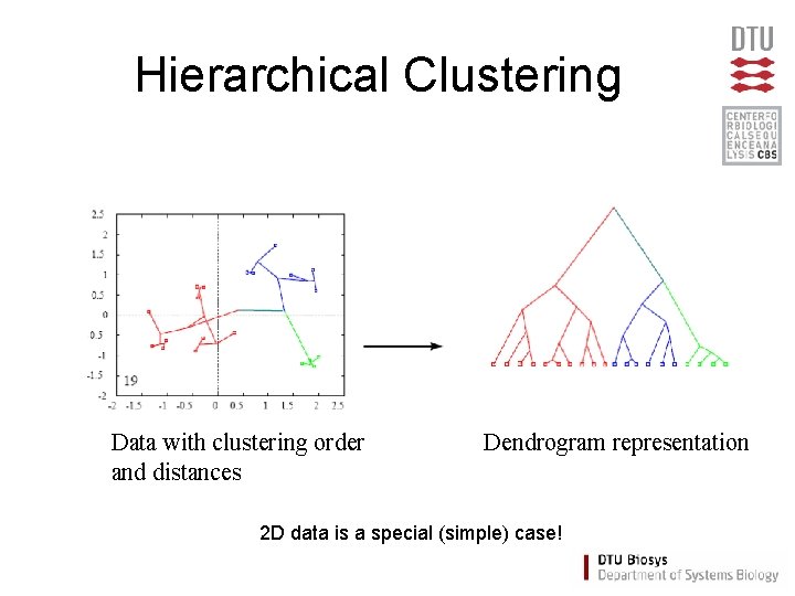
Hierarchical Clustering Data with clustering order and distances Dendrogram representation 2 D data is a special (simple) case!

Hierarchical clustering example: leukemia patients (based on all genes)

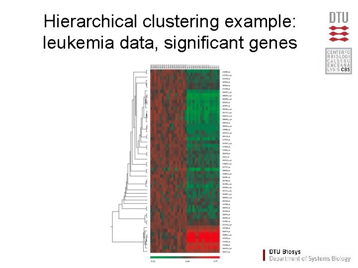
Hierarchical clustering example: leukemia data, significant genes

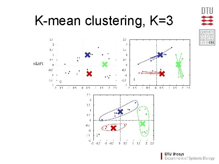
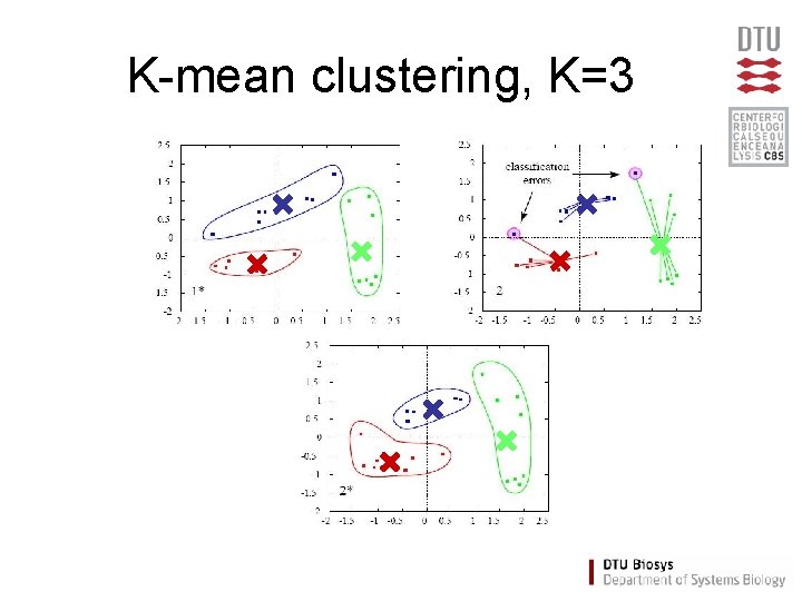
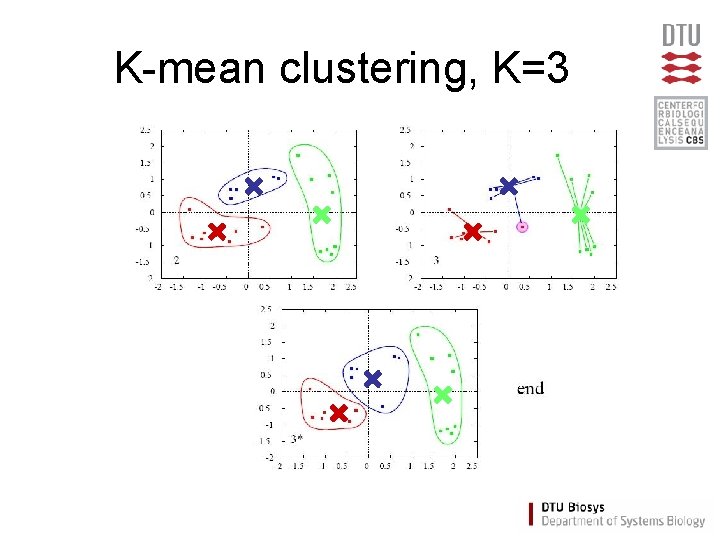
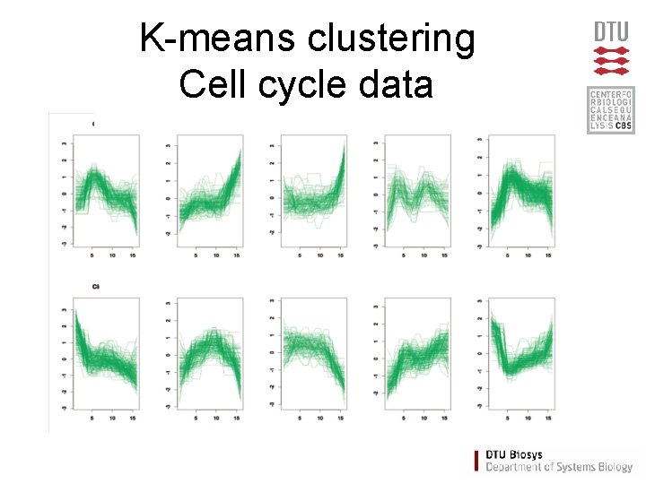
K-mean clustering • Partition data into K clusters • Parameter: Number of clusters (K) must be chosen • Randomilized initialization: – different clusters each time

K-mean - Algorithm • Assign each item a class in 1 to K (randomly) • For each class 1 to K – Calculate the centroid (one of the K-means) – Calculate distance from centroid to each item • Assign each item to the nearest centroid • Repeat until no items are re-assigned (convergence)

K-mean clustering, K=3

K-mean clustering, K=3

K-mean clustering, K=3

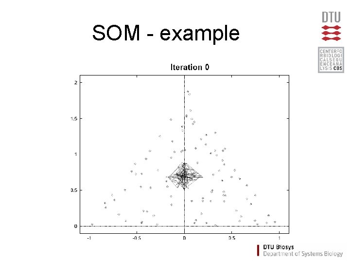
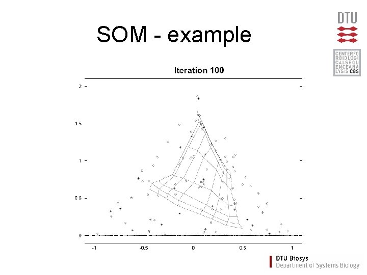
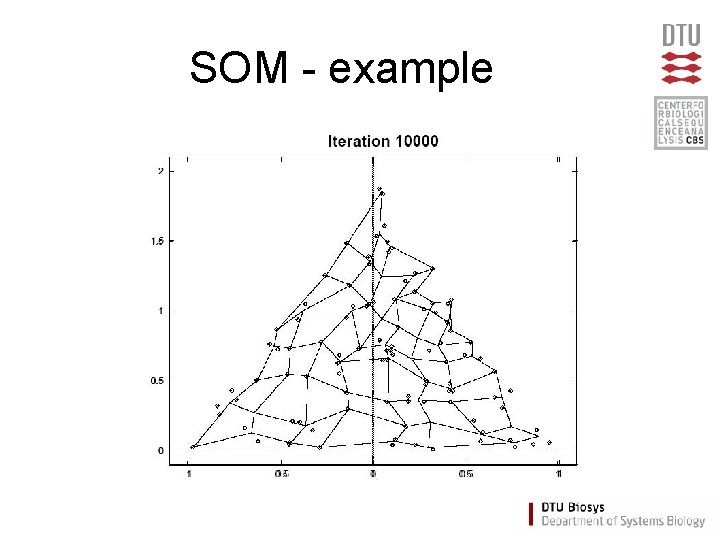
Self Organizing Maps (SOM) • Partitioning method (similar to the K-means method) • Clusters are organized in a two-dimensional grid • Size of grid must be specified – (eg. 2 x 2 or 3 x 3) • SOM algorithm finds the optimal organization of data in the grid

SOM - example

SOM - example

SOM - example

SOM - example

SOM - example

K-means clustering Cell cycle data

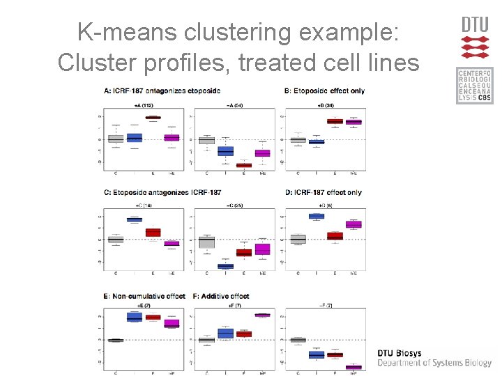
K-means clustering example: Cluster profiles, treated cell lines

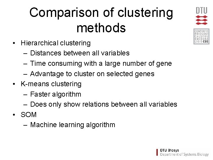
Comparison of clustering methods • Hierarchical clustering – Distances between all variables – Time consuming with a large number of gene – Advantage to cluster on selected genes • K-means clustering – Faster algorithm – Does only show relations between all variables • SOM – Machine learning algorithm

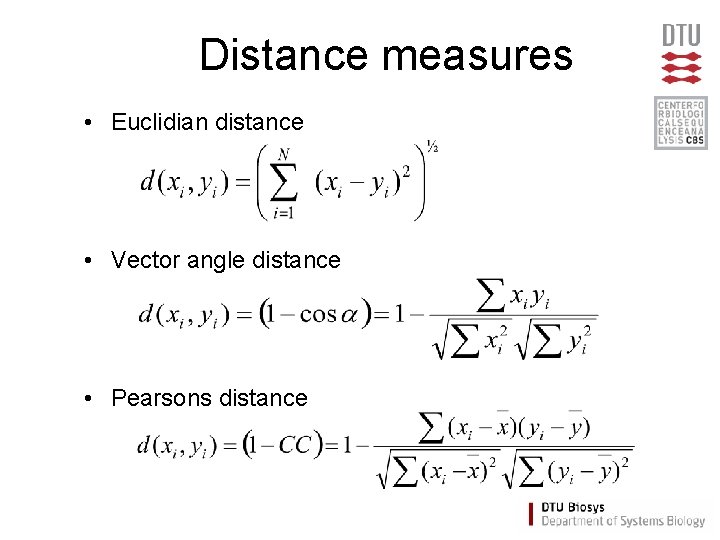
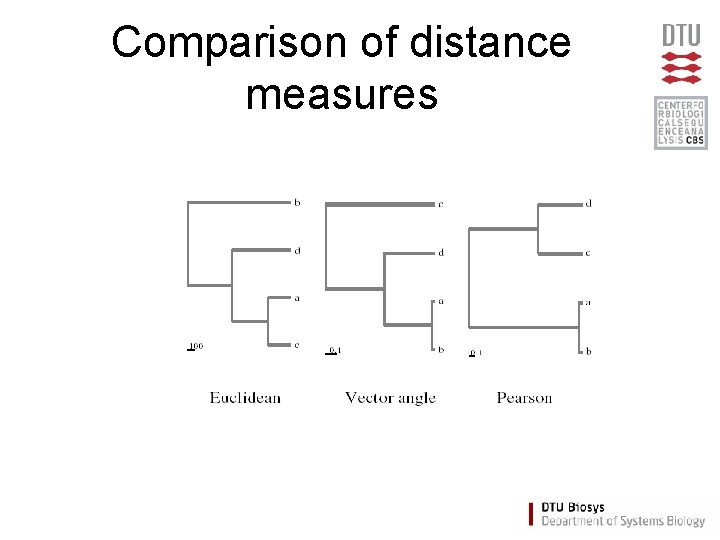
Distance measures • Euclidian distance • Vector angle distance • Pearsons distance

Comparison of distance measures

Summary • Dimension reduction important to visualize data • Methods: – Principal Component Analysis – Clustering • Hierarchical • K-means • Self organizing maps (distance measure important)

Coffee break Next: Exercises in PCA and clustering