Digital topology and crosssection topology for grayscale image

Digital topology and cross-section topology for grayscale image processing M. Couprie A 2 SI lab. , ESIEE Marne-la-Vallée, France www. esiee. fr/a 2 si 1

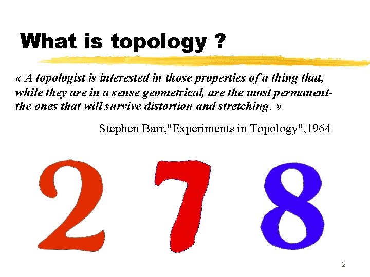
What is topology ? « A topologist is interested in those properties of a thing that, while they are in a sense geometrical, are the most permanentthe ones that will survive distortion and stretching. » Stephen Barr, "Experiments in Topology", 1964 2

Aims of this talk z Present the main notions of digital topology z Show their usefulness in image processing applications z Study some topological properties of digital grayscale images (ie. functions from Zn to Z) z Topology-preserving image transforms z Topology-altering image transforms z Applications to image processing (filtering, segmentation…) 3

Some milestones z. J. C. Maxwell (1870): ‘On hills and dales ’ z. A. Rosenfeld (1970’s): digital topology z. A. Rosenfeld (1980’s): fuzzy digital topology z. S. Beucher (1990): definition of homotopy between grayscale images z. G. Bertrand (1995): cross-section topology 4

Contributors z. Gilles Bertrand z. Michel Couprie z. Laurent Perroton z. Zouina Aktouf (Ph. D student) z. Francisco Nivando Bezerra (Ph. D student) z. Xavier Daragon (Ph. D student) z. Petr Dokládal (Ph. D student) z. Jean-Christophe Everat (Ph. D student) 5

Outline of the talk Part 1 z. Digital topology for binary images z. Applications to graylevel image processing Part 2 z. Cross-section topology for grayscale images z. Topology-altering transforms, applications 6

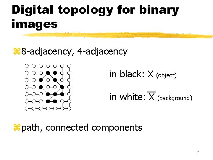
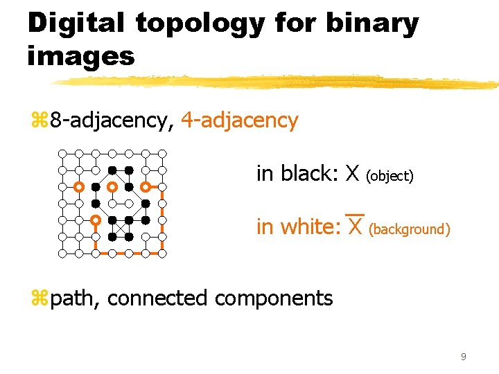
Digital topology for binary images z 8 -adjacency, 4 -adjacency in black: X (object) in white: X (background). zpath, connected components 7

Digital topology for binary images z 8 -adjacency, 4 -adjacency in black: X (object) in white: X (background) . zpath, connected components 8

Digital topology for binary images z 8 -adjacency, 4 -adjacency in black: X (object) in white: X (background) . zpath, connected components 9

Digital topology for binary images z 8 -adjacency, 4 -adjacency in black: X (object) in white: X (background) . zpath, connected components 10

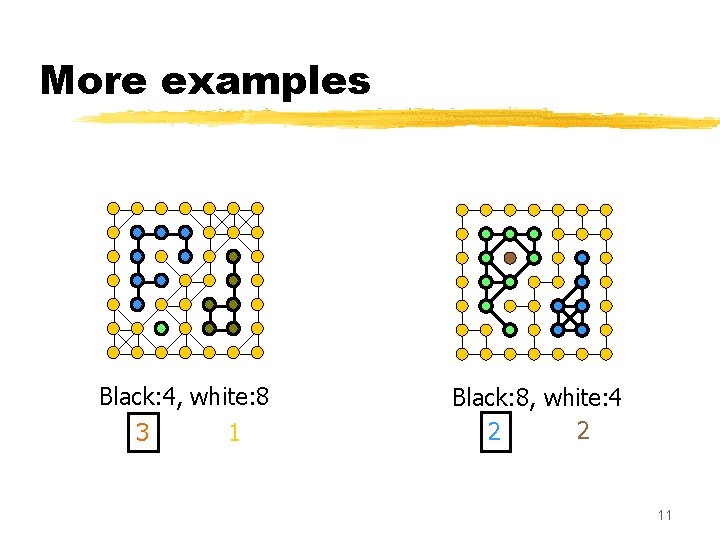
More examples Black: 4, white: 8 3 1 Black: 8, white: 4 2 2 11

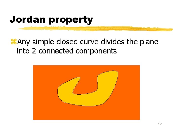
Jordan property z. Any simple closed curve divides the plane into 2 connected components. 12

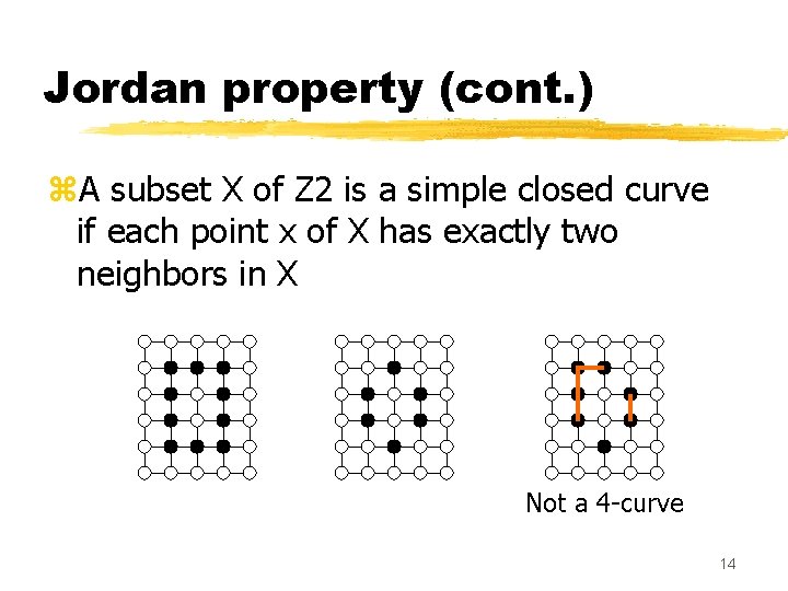
Jordan property (cont. ) z. A subset X of Z 2 is a simple closed curve if each point x of X has exactly two neighbors in X 4 -curve 8 -curve 13

Jordan property (cont. ) z. A subset X of Z 2 is a simple closed curve if each point x of X has exactly two neighbors in X Not a 4 -curve 14

Jordan property (cont. ) z. A subset X of Z 2 is a simple closed curve if each point x of X has exactly two neighbors in X Not an 8 -curve 15

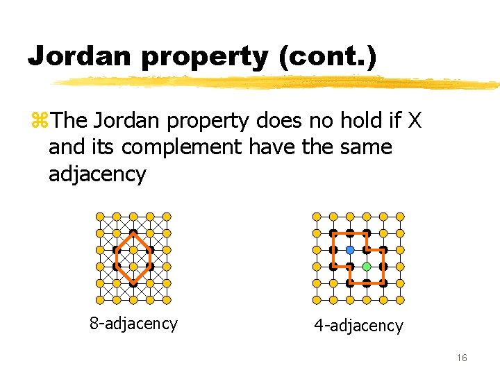
Jordan property (cont. ) z. The Jordan property does no hold if X and its complement have the same adjacency 8 -adjacency 4 -adjacency 16

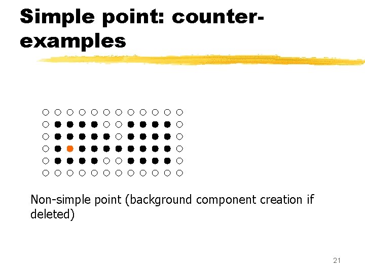
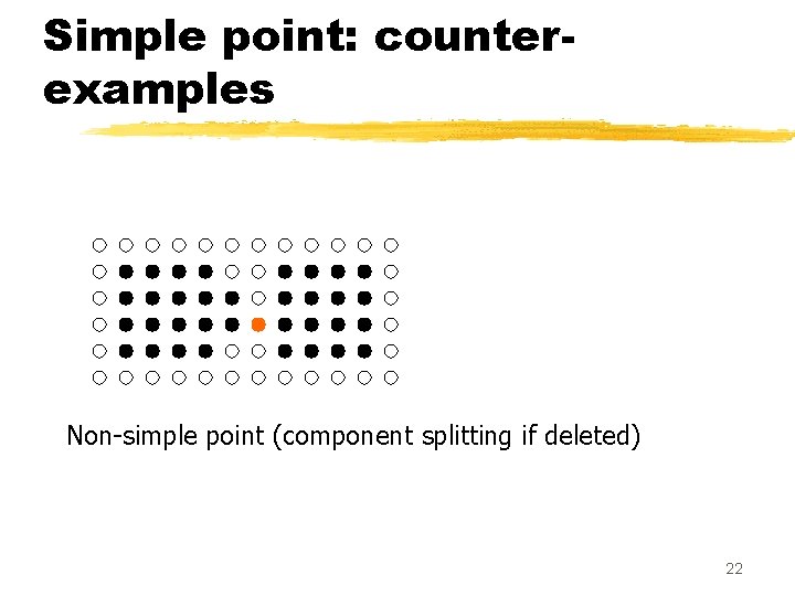
Topology preservation notion of simple point z A topology-preserving transform must preserve the number of connected components of both X and X. z Definition (2 D): A point p is simple (for X) if its modification (addition to X, withdrawal from X) does not change the number of connected components of X and X. 17

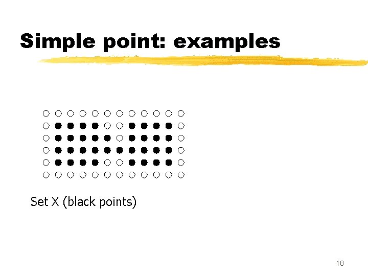
Simple point: examples Set X (black points) 18

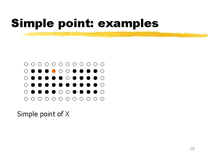
Simple point: examples Simple point of X 19

Simple point: examples Simple point of X 20

Simple point: counterexamples Non-simple point (background component creation if deleted) 21

Simple point: counterexamples Non-simple point (component splitting if deleted) 22

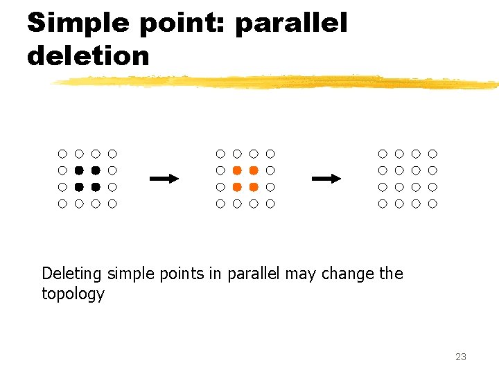
Simple point: parallel deletion Deleting simple points in parallel may change the topology 23

Simple point: local characterization ? 24

Simple point: local characterization ? 25

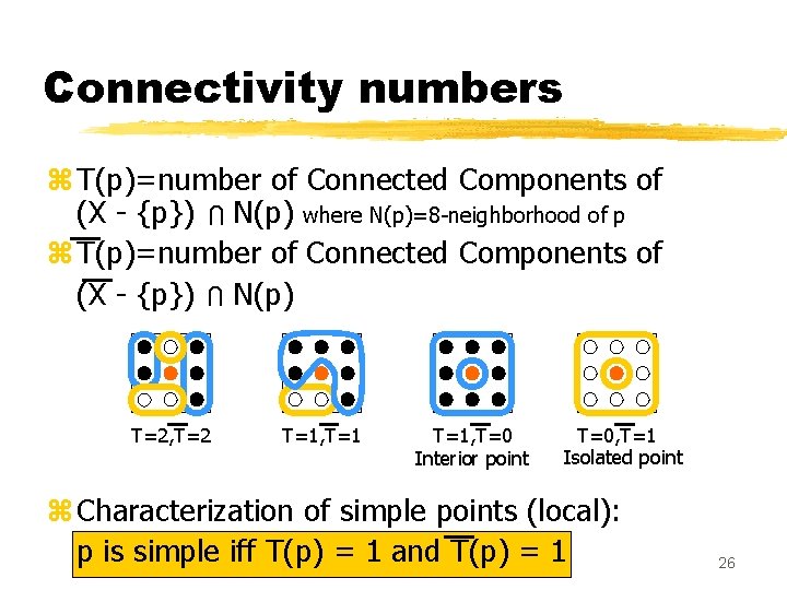
Connectivity numbers z T(p)=number of Connected Components of (X - {p}) N(p) where N(p)=8 -neighborhood of p z T(p)=number of Connected Components of (X - {p}) N(p)A U U T=2, T=2 T=1, T=0 Interior point T=0, T=1 Isolated point z Characterization of simple points (local): p is simple iff T(p) = 1 and T(p) = 1 A 26

Skeletons z We say that Y is a skeleton of X if Y may be obtained from X by sequential deletion of simple points z If Y is a skeleton of X and if Y contains no simple point, then we say that Y is an ultimate skeleton of X z If Y is a skeleton of X and if Y contains only nonsimple points and ‘end points’, then we say that Y is a curve skeleton of X 27

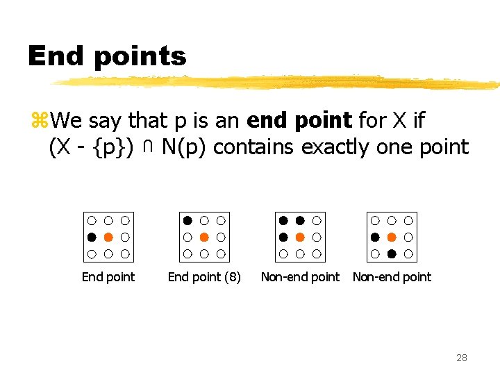
End points z. We say that p is an end point for X if (X - {p}) N(p) contains exactly one point U End point (8) Non-end point 28

Skeletons (examples) End points Original image Curve skeleton Ultimate skeleton 29

Homotopy z. We say that X and Y are homotopic (i. e. they have the same topology) if Y may be obtained from X by sequential addition or deletion of simple points 30

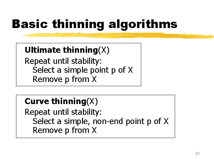
Basic thinning algorithms Ultimate thinning(X) Repeat until stability: Select a simple point p of X Remove p from X Curve thinning(X) Repeat until stability: Select a simple, non-end point p of X Remove p from X 31

Centering skeletons 32

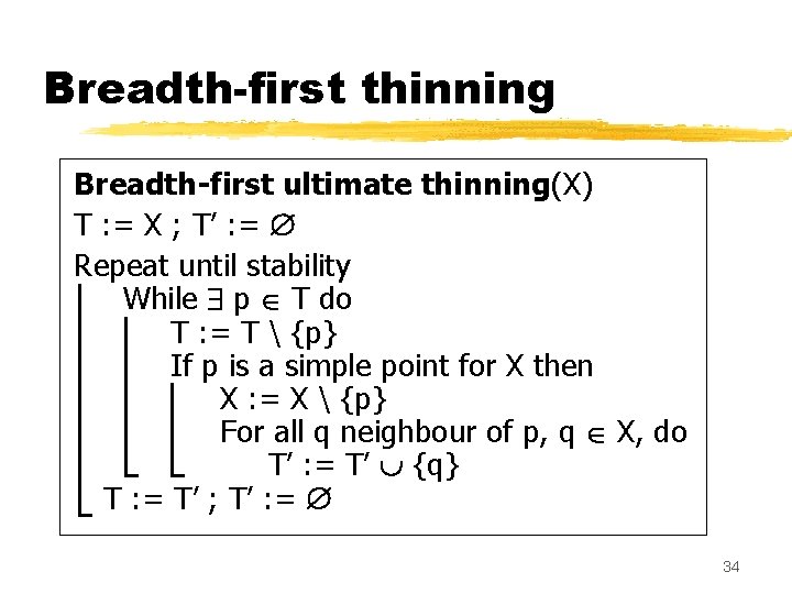
Breadth-first thinning Simple points detected during the 1 st iteration Candidates for the 2 nd iteration 33

Breadth-first thinning Breadth-first ultimate thinning(X) T : = X ; T’ : = Repeat until stability While p T do T : = T {p} If p is a simple point for X then X : = X {p} For all q neighbour of p, q X, do T’ : = T’ {q} T : = T’ ; T’ : = 34

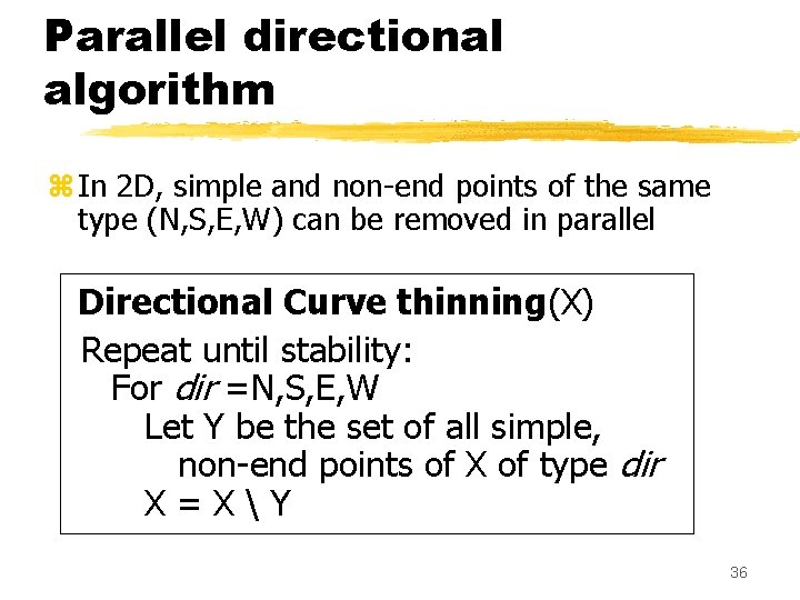
Directional thinning z (only in 2 D) North South East West 35

Parallel directional algorithm z In 2 D, simple and non-end points of the same type (N, S, E, W) can be removed in parallel Directional Curve thinning(X) Repeat until stability: For dir =N, S, E, W Let Y be the set of all simple, non-end points of X of type dir X = X Y 36

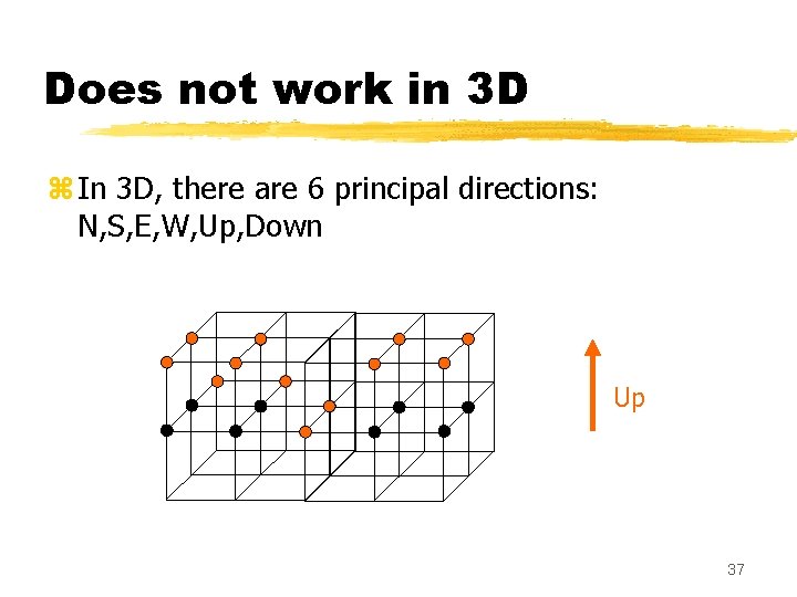
Does not work in 3 D z In 3 D, there are 6 principal directions: N, S, E, W, Up, Down Up 37

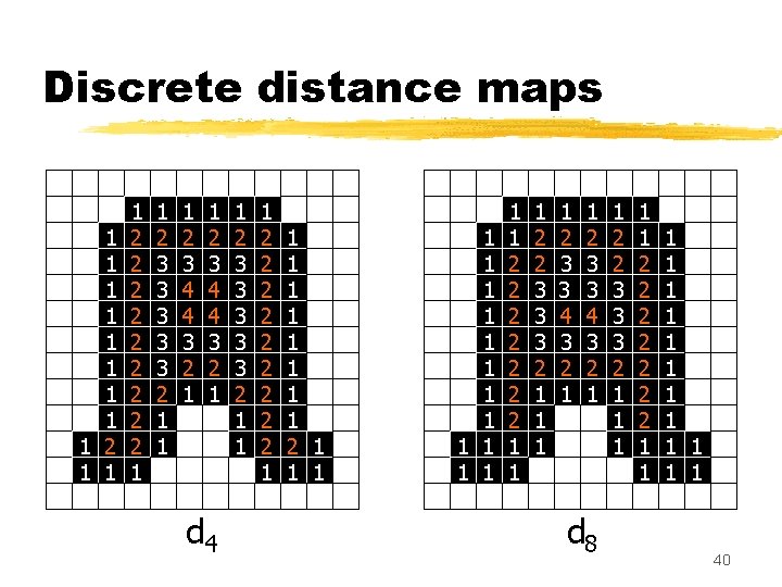
Thinning guided by a distance map z. Let X be a subset of Z 2, the distance map DMX is defined by, for all point p: DMX(p) = min{dist(p, q), q not in X} where dist is a distance (e. g. city block, chessboard, Euclidean) 38

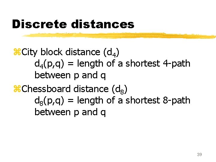
Discrete distances z. City block distance (d 4) d 4(p, q) = length of a shortest 4 -path between p and q z. Chessboard distance (d 8) d 8(p, q) = length of a shortest 8 -path between p and q 39

Discrete distance maps 1 1 1 1 1 2 2 2 2 2 1 1 2 3 3 3 2 1 1 1 2 3 4 4 3 2 1 d 4 1 2 3 3 3 2 1 1 1 2 2 2 2 2 1 1 1 1 1 1 1 2 2 2 2 1 1 1 2 2 3 3 3 2 1 1 2 3 3 4 3 2 1 d 8 1 2 2 3 3 3 2 1 1 1 2 2 2 2 1 1 1 1 40

Discrete and Euclidean distance maps d 8 d 4 de 41

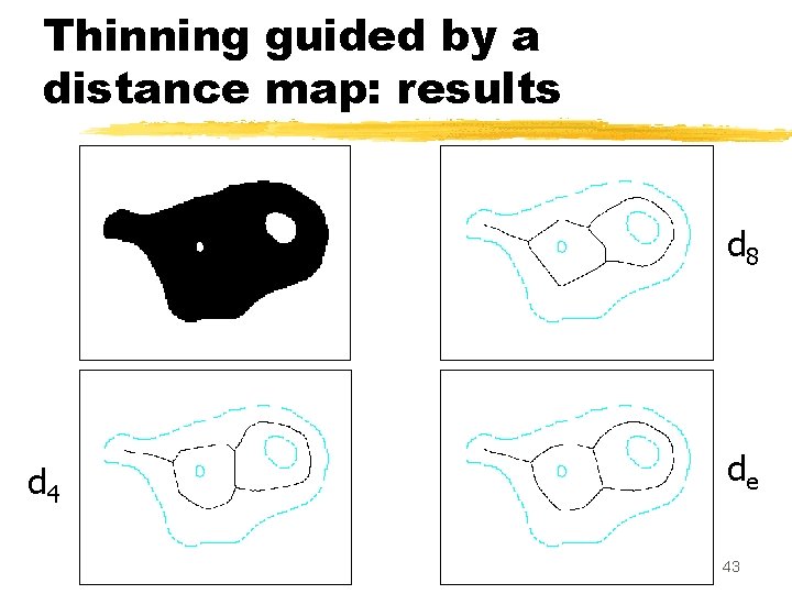
Thinning guided by a distance map: algorithm Ultimate guided thinning(X) Compute the distance map DMX Repeat until stability: Select a simple point p of X such that DMX(p) is minimal Remove p from X Curve guided thinning(X) Id. , replace « simple » by « simple non end » 42

Thinning guided by a distance map: results d 8 d 4 de 43

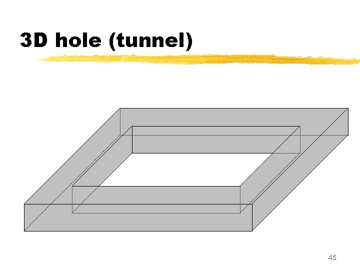
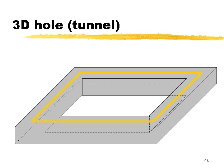
The 3 D case A topology-preserving transform must preserve: - number of connected components of X - number of « holes » (or « tunnels » ) 44

3 D hole (tunnel) 45

3 D hole (tunnel) 46

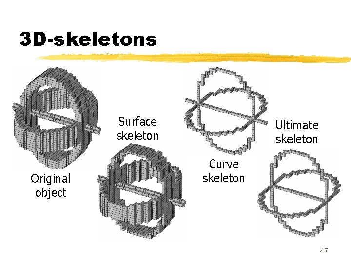
3 D-skeletons Surface skeleton Original object Ultimate skeleton Curve skeleton 47

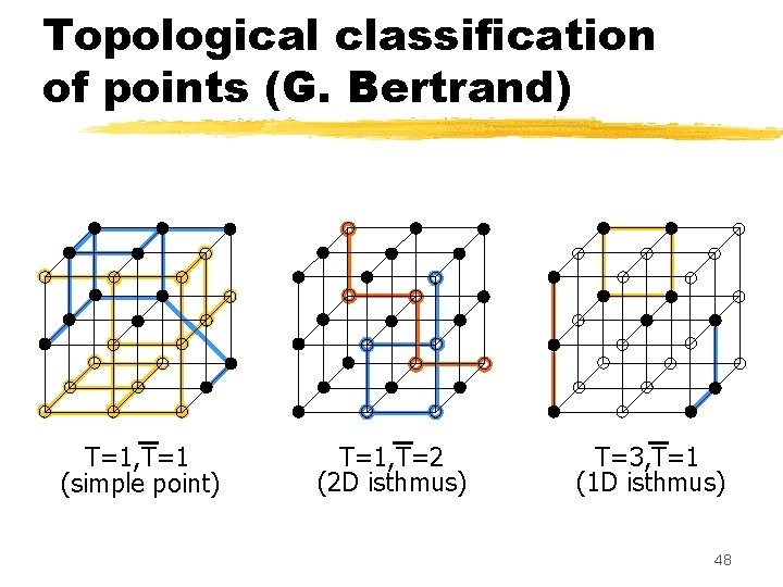
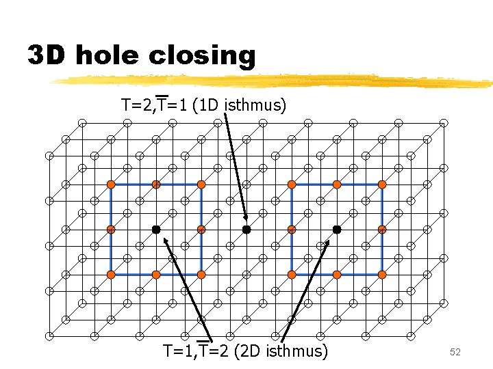
Topological classification of points (G. Bertrand) T=1, T=1 (simple point) T=1, T=2 (2 D isthmus) T=3, T=1 (1 D isthmus) 48

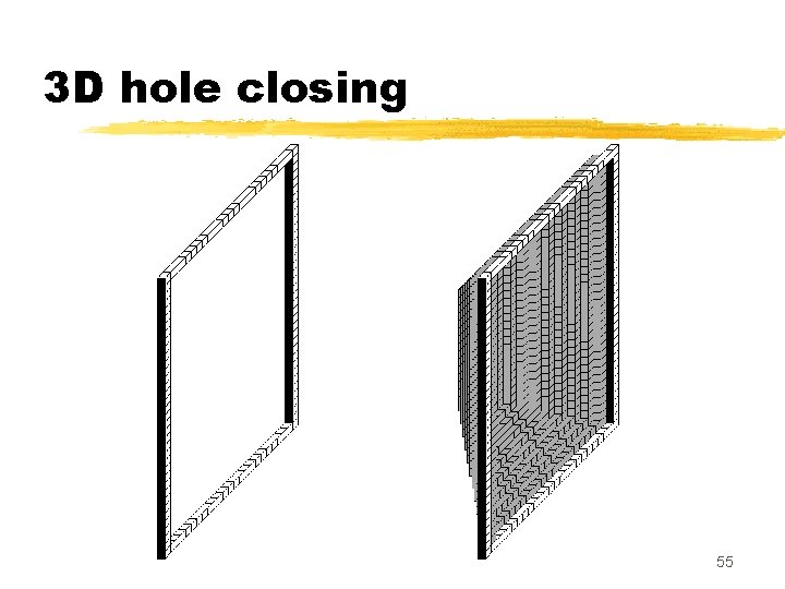
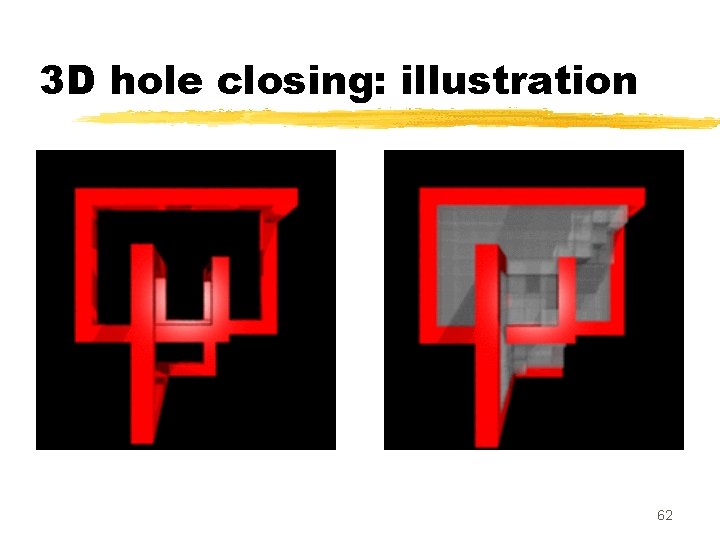
3 D hole closing z. G. Bertrand z. Z. Aktouf (Ph. D) z. L. Perroton 49

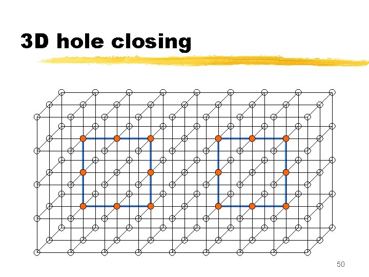
3 D hole closing 50

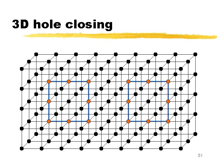
3 D hole closing 51

3 D hole closing T=2, T=1 (1 D isthmus) T=1, T=2 (2 D isthmus) 52

3 D hole closing 53

3 D hole closing algorithm z. Let X be an object and Y be a simply connected set containing X z. We remove iteratively all points x of Y X such that T(x) = 1 (i. e. simple points and 1 D isthmus) 54

3 D hole closing 55

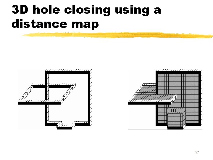
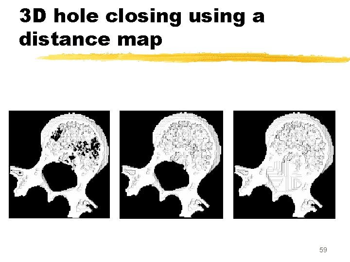
3 D hole closing using a distance map z. The points are processed in an order depending on their distance from X (points far from X are selected first) 56

3 D hole closing using a distance map 57

3 D hole closing using a distance map z. When a point p with T=2 is selected, its removal would create a hole. The value of the distance map for this point (DMX(p)) gives an information on the « size » of the corresponding hole in X. z. We can decide to let a hole open or to close it according to this criterion. 58

3 D hole closing using a distance map 59

3 D hole closing: illustration 60

3 D hole closing: illustration 61

3 D hole closing: illustration 62

Outline of the talk Part 1 z. Digital topology for binary images z. Applications to graylevel image processing Part 2 z. Cross-section topology for grayscale images z. Topology-altering transforms, applications 63

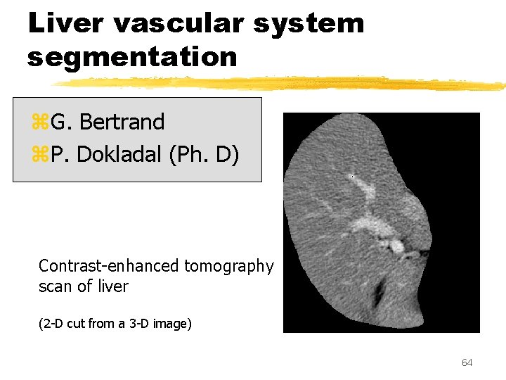
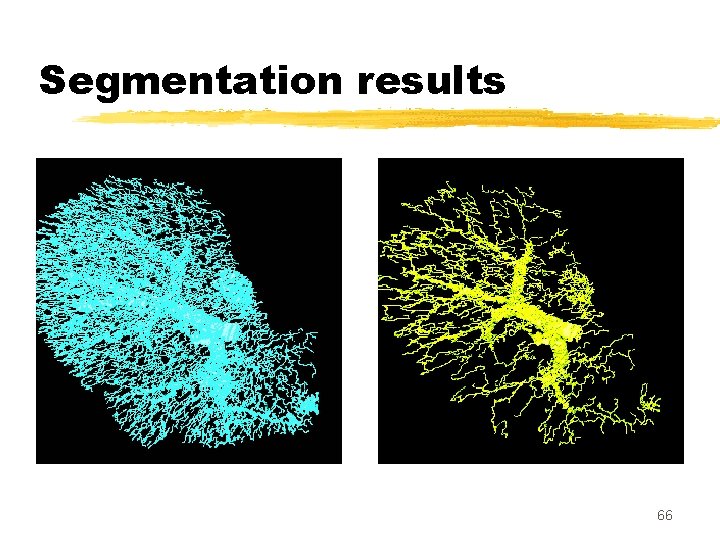
Liver vascular system segmentation z. G. Bertrand z. P. Dokladal (Ph. D) Contrast-enhanced tomography scan of liver (2 -D cut from a 3 -D image) 64

Intensity-guided skeletonization 65

Segmentation results 66

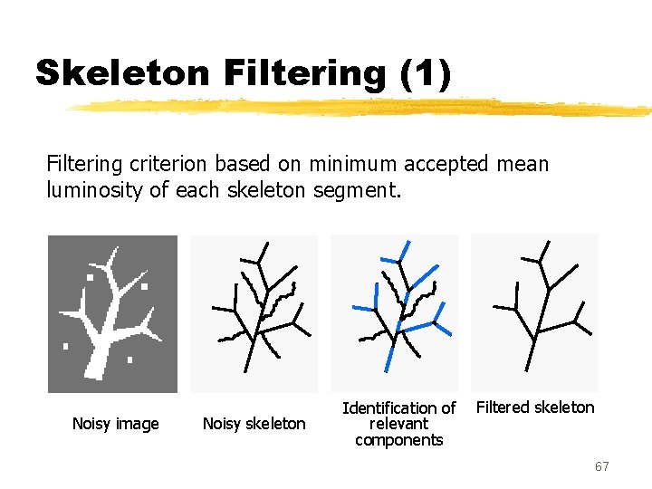
Skeleton Filtering (1) Filtering criterion based on minimum accepted mean luminosity of each skeleton segment. Noisy image Noisy skeleton Identification of Filtered skeleton relevant components 67

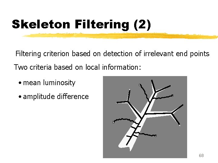
Skeleton Filtering (2) Filtering criterion based on detection of irrelevant end points Two criteria based on local information: • mean luminosity • amplitude difference 68

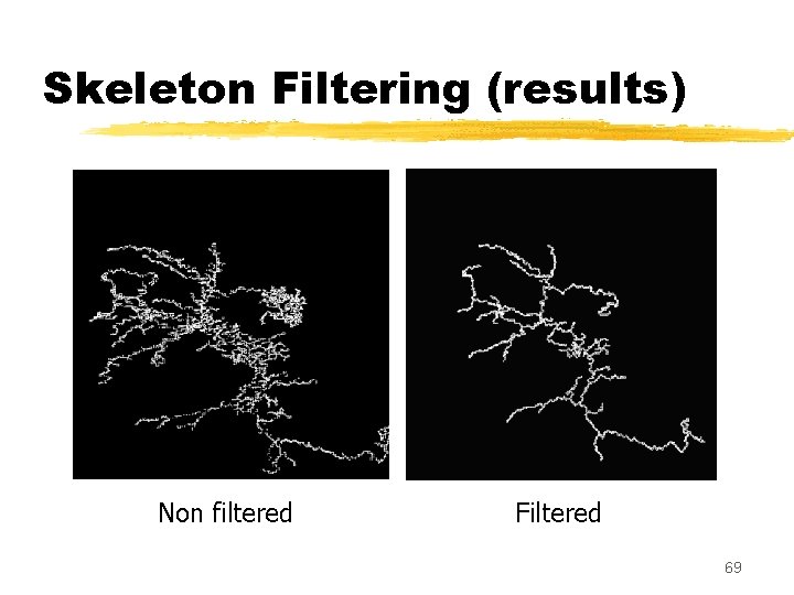
Skeleton Filtering (results) Non filtered Filtered 69

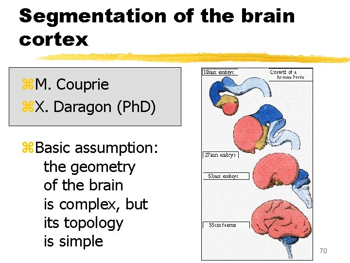
Segmentation of the brain cortex z. M. Couprie z. X. Daragon (Ph. D) z. Basic assumption: the geometry of the brain is complex, but its topology is simple 70

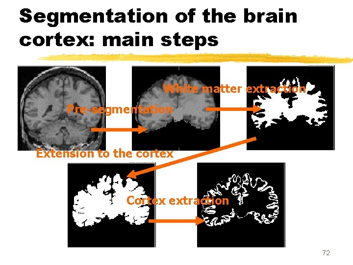
Segmentation of the brain cortex Cortex (gray matter) Cerebrospinal fluid White matter 71

Segmentation of the brain cortex: main steps White matter extraction Pre-segmentation Extension to the cortex Cortex extraction 72

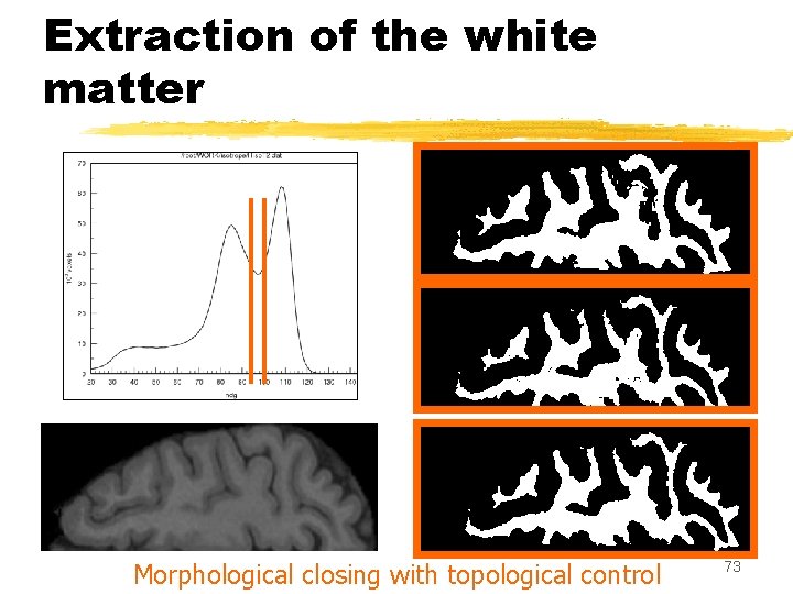
Extraction of the white matter Morphological closing with topological control 73

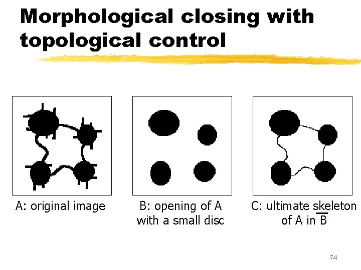
Morphological closing with topological control A: original image B: opening of A with a small disc C: ultimate skeleton of A in B 74

Extension to the cortex W. M. 75

Extension to the cortex: use of a distance map Section of the 3 D segmentation of the white matter Section of its 3 D distance map (limited to distances < 1 cm) 76

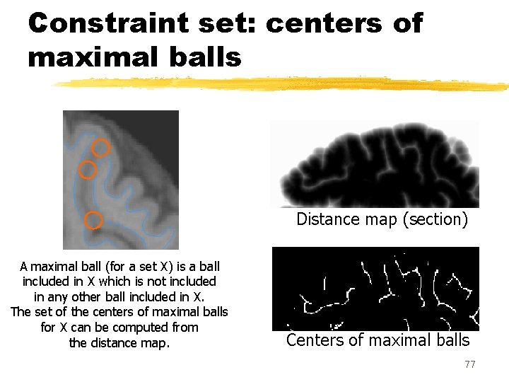
Constraint set: centers of maximal balls Distance map (section) A maximal ball (for a set X) is a ball included in X which is not included in any other ball included in X. The set of the centers of maximal balls for X can be computed from the distance map. Centers of maximal balls 77

Results (sections of 3 D images) Without constraint set With constraint set 78

Results (3 D view) Without constraint set With constraint set 79

Results (3 D view) White matter Cortex 80

Conclusion (1 st part) z. Image simplification with topology preservation z. Controled topology modification z. Binary topological operators guided by a distance map or by a grayscale image z. Efficient implementations 81

Outline of the talk Part 1 z. Digital topology for binary images z. Applications to graylevel image processing Part 2 z. Cross-section topology for grayscale images z. Topology-altering transforms, applications 82

Cross-section topology z. G. Bertrand z. M. Couprie z. J. C. Everat (Ph. D) z. F. N. Bezerra (Ph. D) 83

Cross-section topology z. Basic idea: consider the topology of each cross-section (threshold) of a function. z. Given a function F (Z 2 Z) and k in Z, we define the cross-section Fk as the set of points p of Z 2 such that F(p) k. z. We say that two functions F and G are homotopic if, for every k in Z, Fk and Gk are homotopic (in the binary sense) 84

Homotopy: an illustration F(x, y) y G(x, y) y x x F 3 G 3 F 2 G 2 F 1 G 1 85

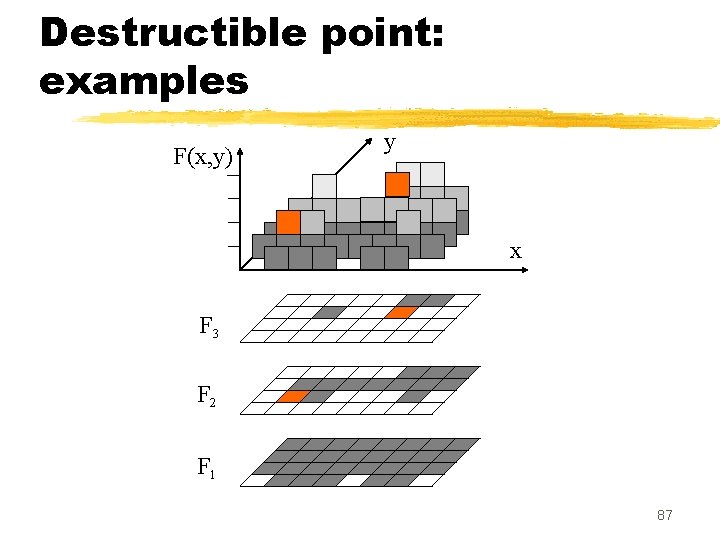
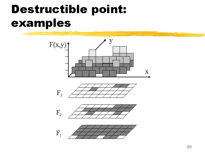
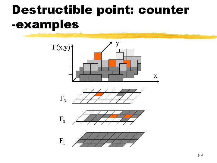
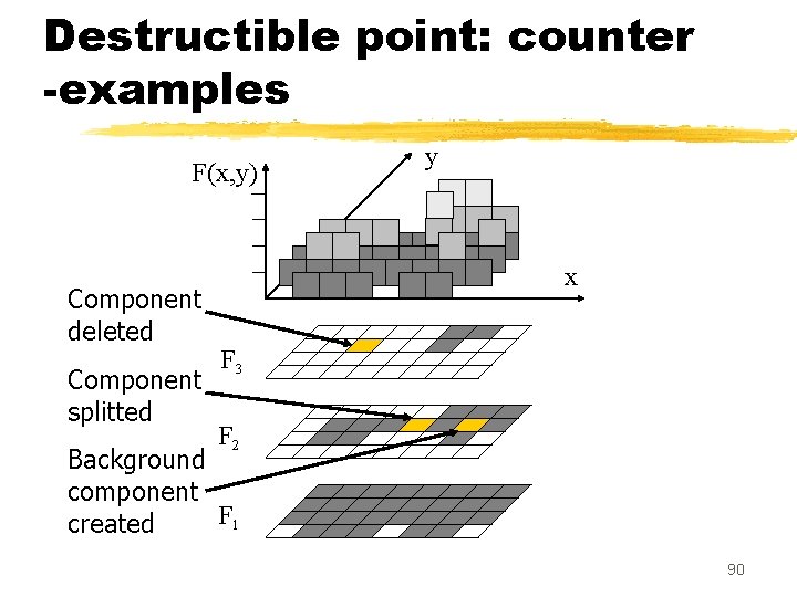
Destructible point (G. Bertrand) z. Definition: a point p is destructible (for F) if it is simple for Fk, with k = F(p) . z. Property: p is destructible iff its value may be lowered by one without changing the topology of any cross-section. z. Definition: a point p is constructible (for F) if it is destructible for -F (duality) 86

Destructible point: examples F(x, y) y x F 3 F 2 F 1 87

Destructible point: examples F(x, y) y x F 3 F 2 F 1 88

Destructible point: counter -examples F(x, y) y x F 3 F 2 F 1 89

Destructible point: counter -examples F(x, y) Component deleted Component splitted y x F 3 F 2 Background component F 1 created 90

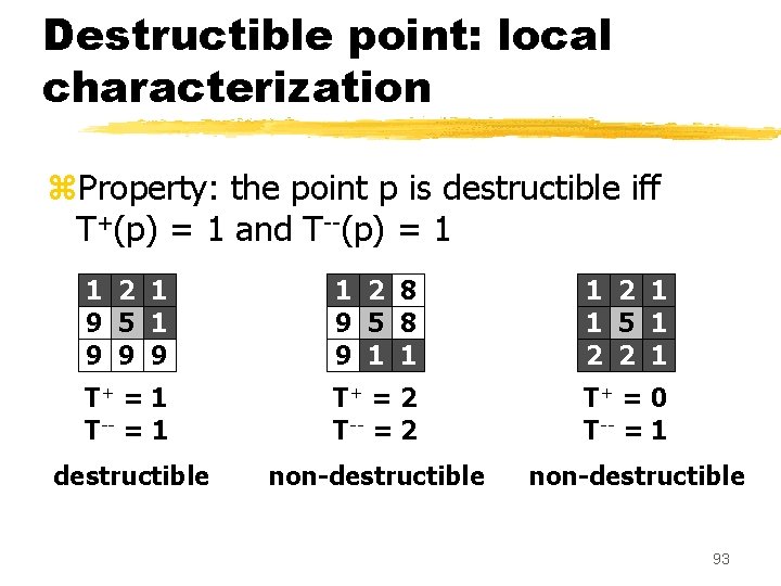
Connectivity numbers z N+(p) = {q in N(p), F(q) F(p)} z T+(p) = number of Conn. Comp. of N+(p) . z N--(p) = {q in N(p), F(q) < F(p)} z T--(p) = number of Conn. Comp. of N--(p) . z N++, T++, N-, T- : similar z If an adjacency relation (eg. 4) is chosen for T+, T++, then the other adjacency (8) must be used for T-, T-- 91

Connectivity numbers: examples 1 2 1 9 5 1 9 9 9 1 2 8 9 5 8 9 1 1 1 2 1 1 5 1 2 2 1 T+ = 1 T-- = 1 T+ = 2 T-- = 2 T+ = 0 T-- = 1 92

Destructible point: local characterization z. Property: the point p is destructible iff T+(p) = 1 and T--(p) = 1 1 2 1 9 5 1 9 9 9 1 2 8 9 5 8 9 1 1 1 2 1 1 5 1 2 2 1 T+ = 1 T-- = 1 T+ = 2 T-- = 2 T+ = 0 T-- = 1 destructible non-destructible 93

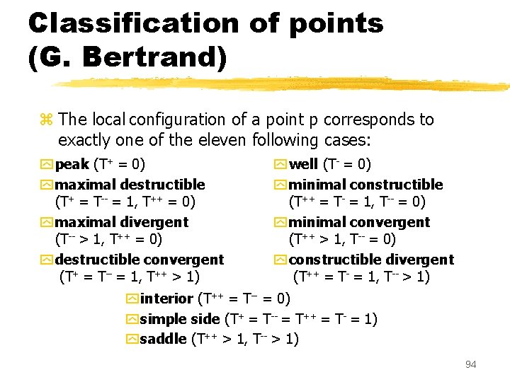
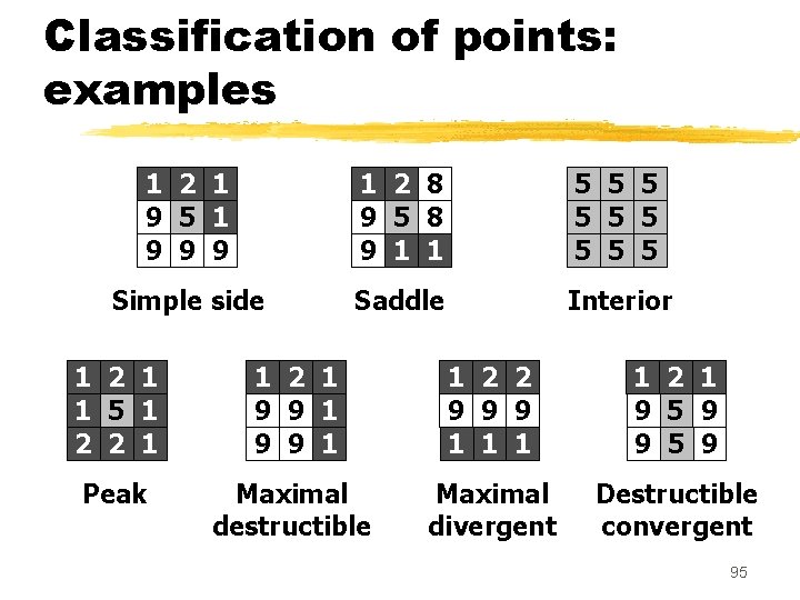
Classification of points (G. Bertrand) z The local configuration of a point p corresponds to exactly one of the eleven following cases: y peak (T+ = 0) y maximal destructible (T+ = T-- = 1, T++ = 0) y maximal divergent (T-- > 1, T++ = 0) y destructible convergent (T+ = T-- = 1, T++ > 1) y well (T- = 0) y minimal constructible (T++ = T- = 1, T-- = 0) y minimal convergent (T++ > 1, T-- = 0) y constructible divergent (T++ = T- = 1, T-- > 1) y interior (T++ = T-- = 0) y simple side (T+ = T-- = T++ = T- = 1) y saddle (T++ > 1, T-- > 1) 94

Classification of points: examples 1 2 1 9 5 1 9 9 9 1 2 8 9 5 8 9 1 1 5 5 5 5 5 Simple side Saddle Interior 1 2 1 1 5 1 2 2 1 1 2 1 9 9 1 1 2 2 9 9 9 1 1 2 1 9 5 9 Peak Maximal destructible Maximal divergent Destructible convergent 95

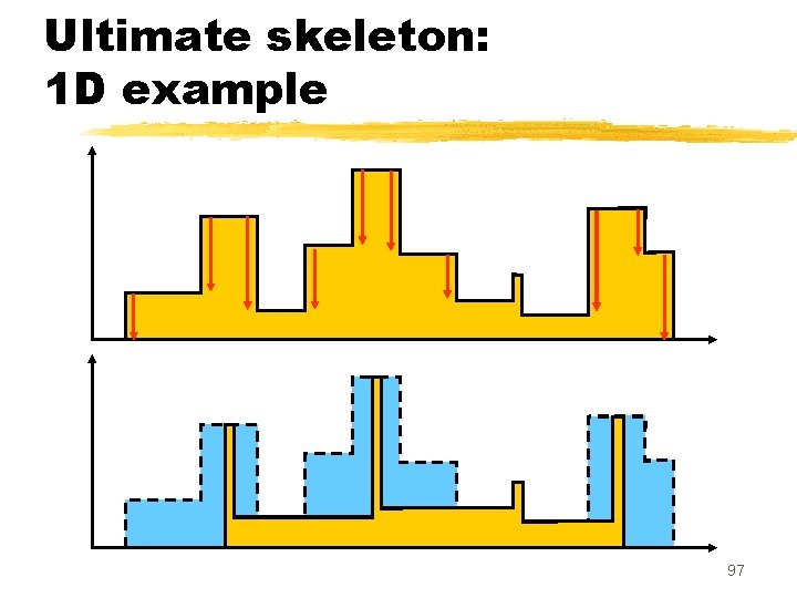
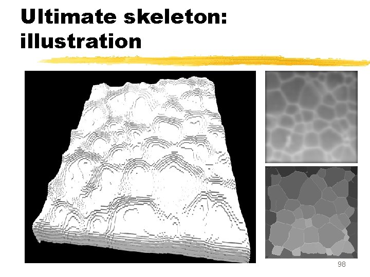
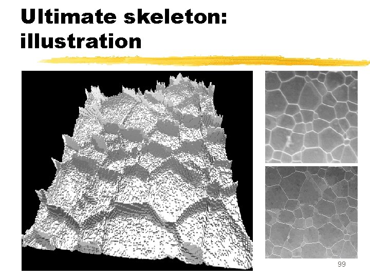
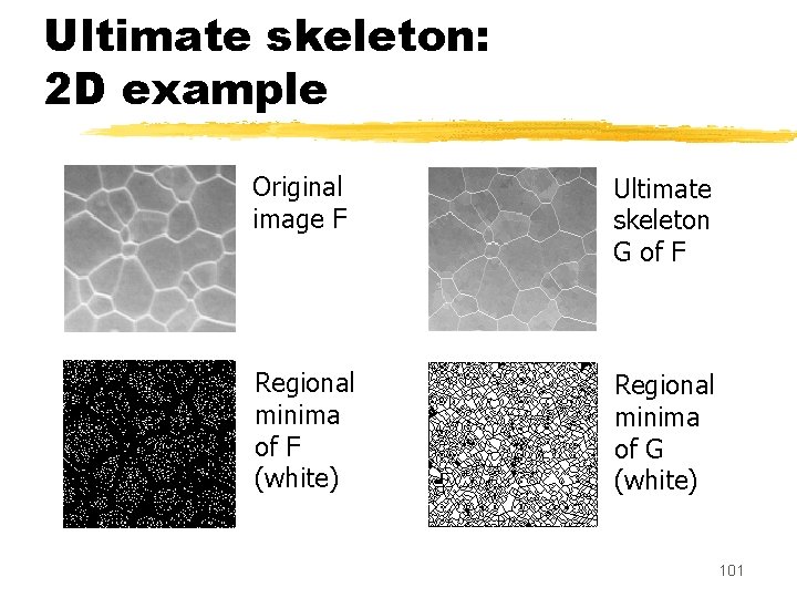
Grayscale skeletons z. We say that G is a skeleton of F if G may be obtained from F by sequential lowering of destructible points. . z. If G is a skeleton of F and if G contains no destructible point, then we say that G is an ultimate skeleton of F 96

Ultimate skeleton: 1 D example 97

Ultimate skeleton: illustration 98

Ultimate skeleton: illustration 99

Ultimate skeleton: 1 D example Regional minima 100

Ultimate skeleton: 2 D example Original image F Ultimate skeleton G of F Regional minima of F (white) Regional minima of G (white) 101

( 102

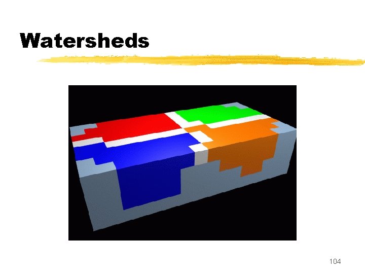
Watersheds z. Powerful segmentation operator from the field of Mathematical Morphology z. Introduced as a tool for segmenting grayscale images by S. Beucher and C. Lantuejoul in the 70 s z. Efficient algorithms based on immersion simulation were proposed by L. Vincent, F. Meyer, P. Soille (and others) in the 90 s 103

Watersheds 104

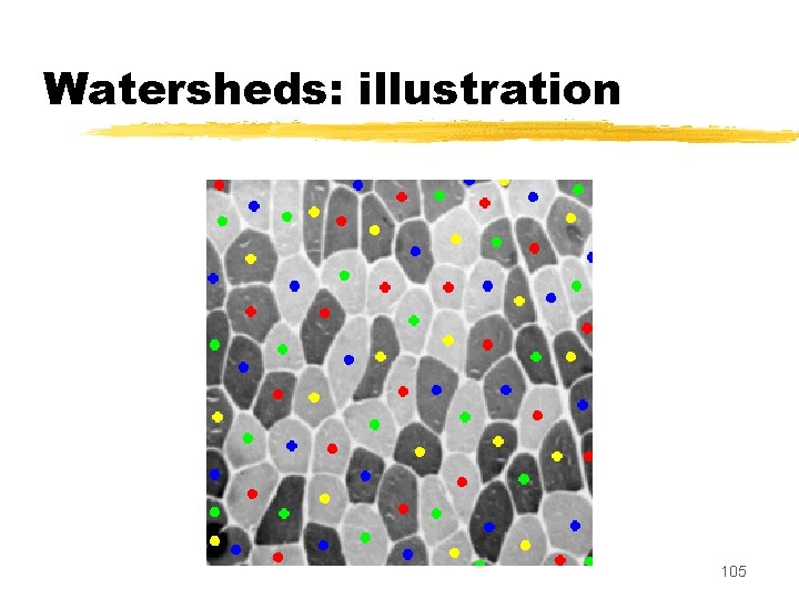
Watersheds: illustration 105

) 106

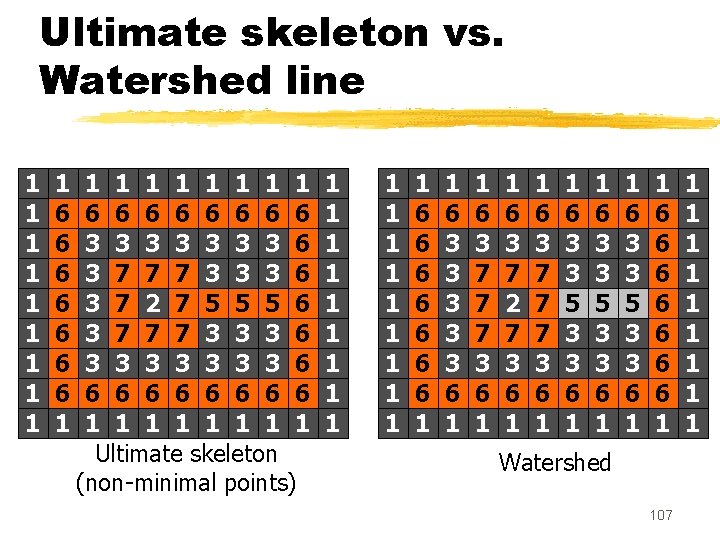
Ultimate skeleton vs. Watershed line 1 1 1 1 1 6 6 6 6 3 3 3 3 6 3 7 7 7 3 3 3 6 3 7 2 7 5 5 5 6 3 7 7 7 3 3 3 6 3 3 3 3 6 6 6 6 6 1 1 1 1 Ultimate skeleton (non-minimal points) 1 1 1 1 1 6 6 6 6 1 1 6 3 3 3 6 1 1 6 3 7 7 7 3 6 1 1 6 3 7 2 7 3 6 1 1 6 3 7 7 7 3 6 1 1 6 3 3 5 3 3 6 1 1 6 6 6 6 1 Watershed 107 1 1 1 1 1

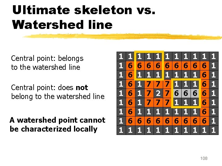
Ultimate skeleton vs. Watershed line Central point: belongs to the watershed line Central point: does not belong to the watershed line A watershed point cannot be characterized locally 1 1 1 1 1 6 6 6 6 1 1 1 1 1 6 1 7 7 7 1 6 1 7 2 7 1 6 1 7 7 7 1 6 1 1 6 1 1 6 1 1 6 6 6 6 1 108 1 1 1 1 1

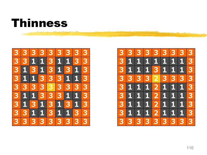
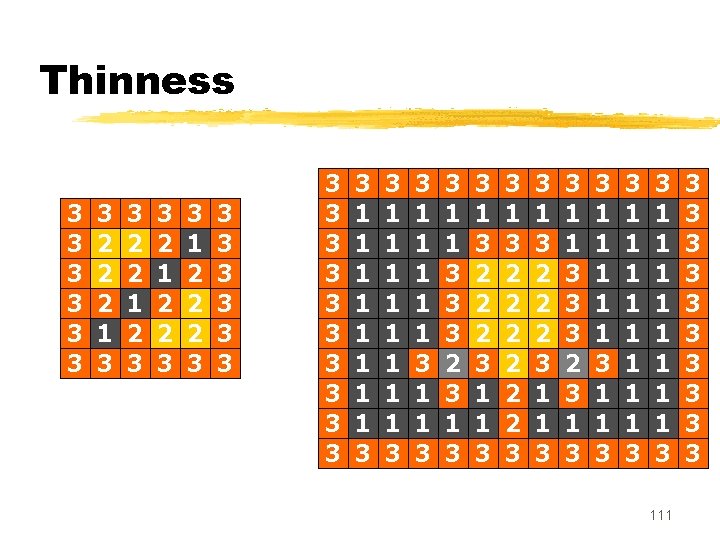
Thinness z. In the previous examples, the set of nonminimal points of an ultimate skeleton was « thin » (a set X is thin if it contains no interior point). Is it always true ? z. The answer is no, as shown by the following counter-examples. 109

Thinness 3 3 3 1 1 3 3 3 1 3 1 3 3 1 1 3 3 3 1 1 3 3 3 1 1 3 3 1 3 1 3 3 3 1 1 3 3 3 3 3 3 1 1 1 1 3 3 1 1 1 1 3 3 1 3 2 2 2 3 3 1 1 1 1 3 3 1 1 1 1 3 3 3 3 3 110

Thinness 3 3 3 3 2 2 2 1 3 3 2 2 1 2 3 3 2 1 2 2 3 3 1 2 2 2 3 3 3 3 3 1 1 1 1 3 3 1 1 1 3 3 3 2 3 1 3 2 2 2 3 1 1 3 3 1 3 2 2 2 3 1 1 3 3 3 2 3 1 3 3 1 1 1 3 3 1 1 1 1 3 111 3 3 3 3 3

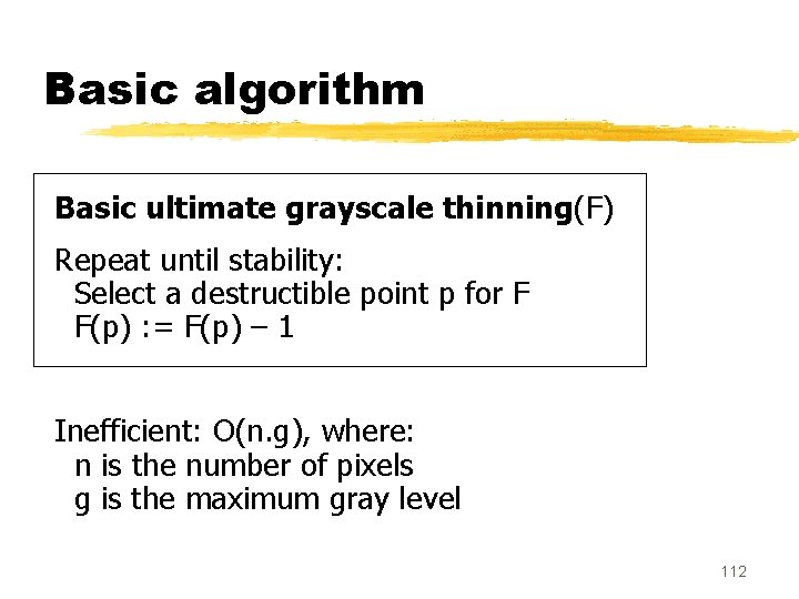
Basic algorithm Basic ultimate grayscale thinning(F) Repeat until stability: Select a destructible point p for F F(p) : = F(p) – 1 Inefficient: O(n. g), where: n is the number of pixels g is the maximum gray level 112

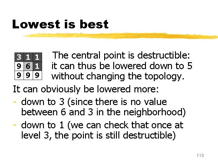
Lowest is best The central point is destructible: 3 1 1 9 it can thus be lowered down to 5 6 1 9 without changing the topology. 9 9 It can obviously be lowered more: - down to 3 (since there is no value between 6 and 3 in the neighborhood) - down to 1 (we can check that once at level 3, the point is still destructible) 113

Two special values If p is destructible, we define: -(p)=highest value strictly lower than F(p) in the neighborhood of p -(p)=lowest value down to which F(p) can be lowered without changing the topology 3 1 1 9 6 1 9 9 9 Here: -(p)=3 (p)=1 114

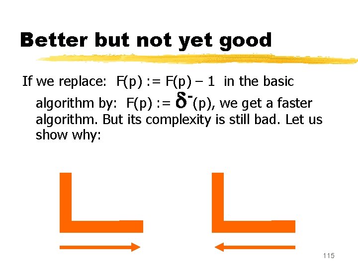
Better but not yet good If we replace: F(p) : = F(p) – 1 in the basic algorithm by: F(p) : = (p), we get a faster algorithm. But its complexity is still bad. Let us show why: 115

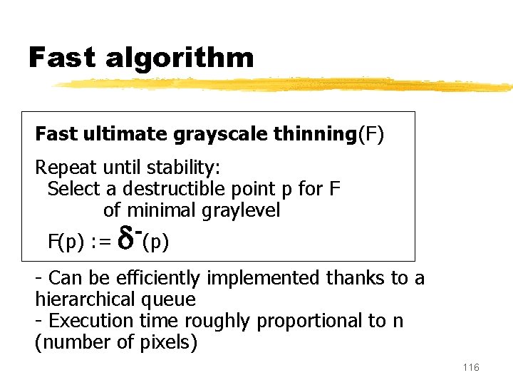
Fast algorithm Fast ultimate grayscale thinning(F) Repeat until stability: Select a destructible point p for F of minimal graylevel F(p) : = (p) - Can be efficiently implemented thanks to a hierarchical queue - Execution time roughly proportional to n (number of pixels) 116

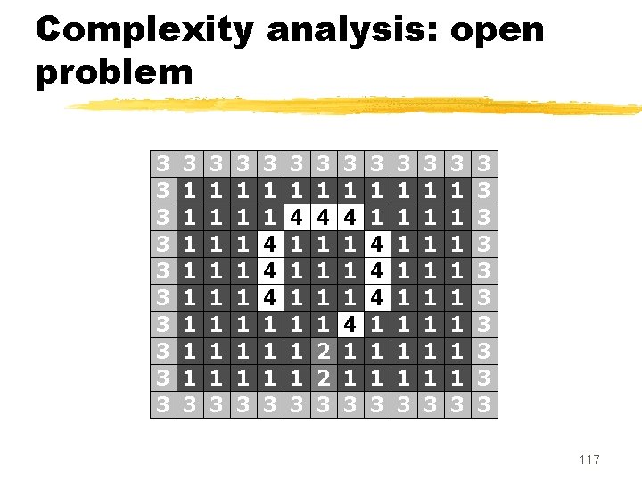
Complexity analysis: open problem 3 3 3 1 1 1 1 3 3 1 1 1 1 3 3 1 1 4 4 4 1 1 1 3 3 1 4 3 2 1 2 3 1 3 2 1 1 4 1 1 3 3 1 4 3 2 1 2 3 1 2 2 3 3 1 4 3 2 1 2 3 1 3 2 1 4 1 1 3 3 1 1 4 4 4 1 1 1 3 3 1 1 1 1 3 3 1 1 1 1 3 3 3 117

Outline of the talk Part 1 z. Digital topology for binary images z. Applications to graylevel image processing Part 2 z. Cross-section topology for grayscale images z. Topology-altering transforms, applications 118

Topology-altering transforms, applications z. G. Bertrand z. M. Couprie z. J. C. Everat (Ph. D) z. F. N. Bezerra (Ph. D) 119

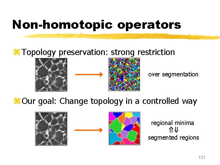
Altering the topology z. Control over topology modification. z. Criteria: y. Local contrast : notion of -skeleton y. Regional contrast : regularization y. Size : topological filtering y. Topology : crestoration 120

Non-homotopic operators z Topology preservation: strong restriction over segmentation z Our goal: Change topology in a controlled way regional minima segmented regions 121

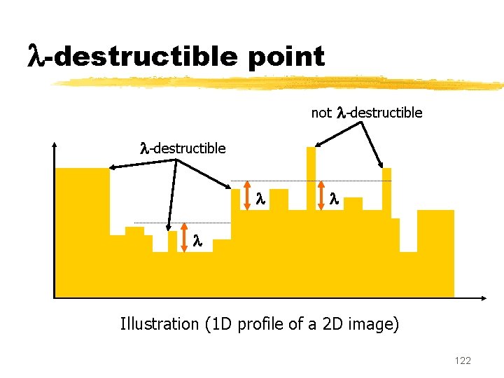
-destructible point not -destructible Illustration (1 D profile of a 2 D image) 122

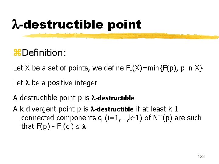
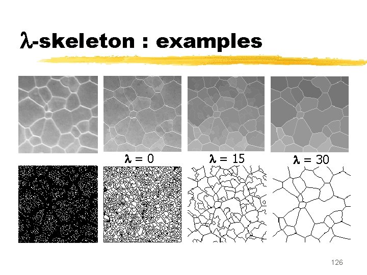
-destructible point z. Definition: Let X be a set of points, we define F-(X)=min{F(p), p in X} Let be a positive integer A destructible point p is -destructible A k-divergent point p is -destructible if at least k-1 connected components ci (i=1, …, k-1) of N--(p) are such that F(p) - F-(ci) 123

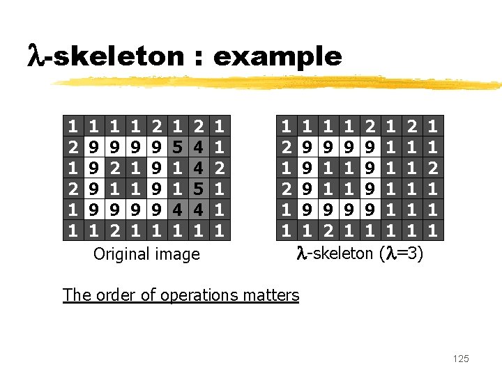
-skeleton . z. We say that G is a -skeleton of F if G may be obtained from F by sequential lowering of -destructible or peak points 124

-skeleton : example 1 2 1 1 1 2 9 9 5 4 9 2 1 9 1 4 9 1 1 9 1 5 9 9 4 4 1 2 1 1 Original image 1 1 2 1 1 1 1 2 1 2 1 9 9 1 1 1 9 1 1 2 9 1 1 1 9 9 1 1 2 1 1 1 -skeleton ( =3) The order of operations matters 125

-skeleton : examples = 0 = 15 = 30 126

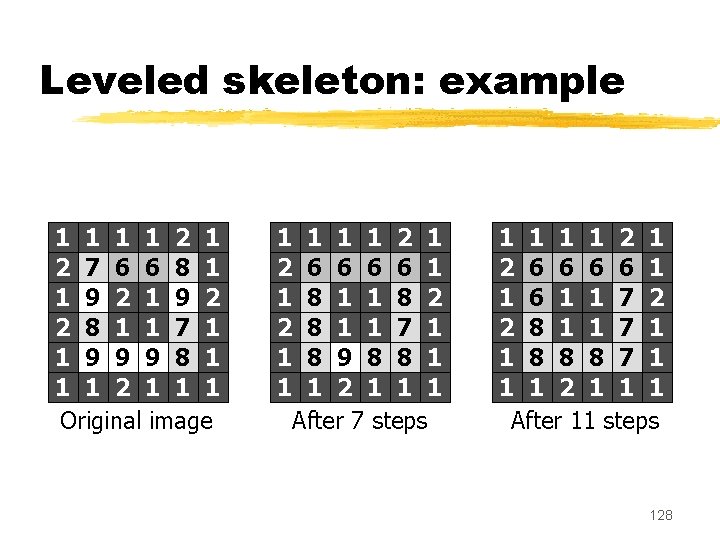
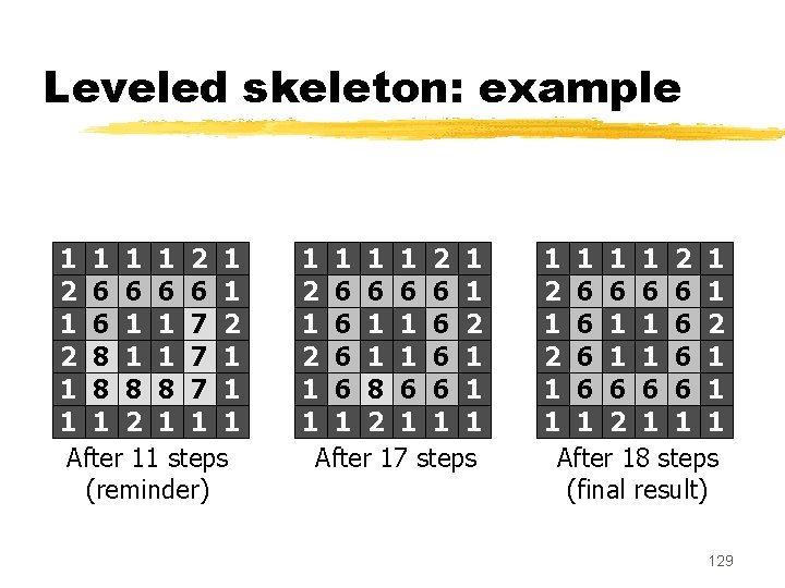
Leveled skeleton z. We say that G is a leveled skeleton of F if G may be obtained from F by sequential lowering of destructible or peak points. 127

Leveled skeleton: example 1 1 2 1 2 7 6 6 8 1 1 9 2 2 8 1 1 7 1 1 9 9 9 8 1 1 1 2 1 1 1 Original image 1 1 2 1 2 6 6 1 1 8 2 2 8 1 1 7 1 1 8 9 8 8 1 1 1 2 1 1 1 After 7 steps 1 1 2 1 2 6 6 1 1 7 2 2 8 1 1 7 1 1 8 8 8 7 1 1 1 2 1 1 1 After 11 steps 128

Leveled skeleton: example 1 1 2 1 2 6 6 1 1 7 2 2 8 1 1 7 1 1 8 8 8 7 1 1 1 2 1 1 1 After 11 steps (reminder) 1 1 2 1 2 6 6 1 1 6 2 2 6 1 1 6 8 6 6 1 1 1 2 1 1 1 After 17 steps 1 1 2 1 2 6 6 1 1 6 2 2 6 1 1 6 6 1 1 1 2 1 1 1 After 18 steps (final result) 129

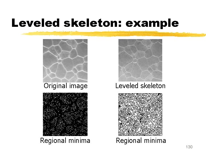
Leveled skeleton: example Original image Leveled skeleton Regional minima 130

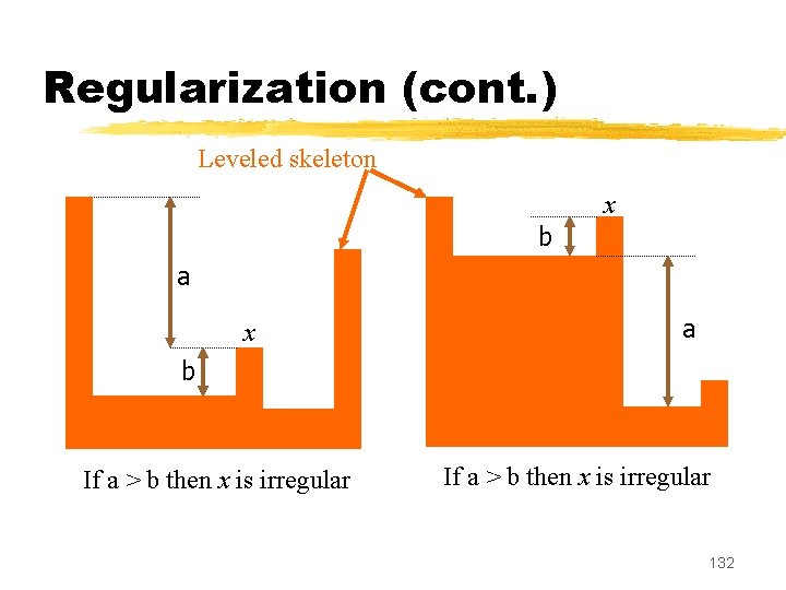
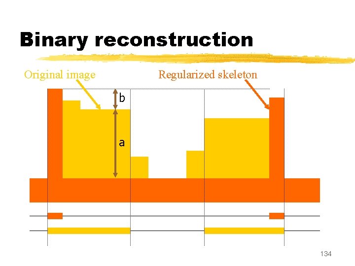
Regularization z. In a leveled skeleton, the regional minima are separated by ‘thin crest lines’ . z. The graylevel on these lines correspond to the ‘altitude of the lowest pass connecting two neighboring minima’ (in the skeleton, and in the original image as well) . z. This allows to detect and modify ‘irregular crest points’ 131

Regularization (cont. ) Leveled skeleton x b a x a b If a > b then x is irregular 132

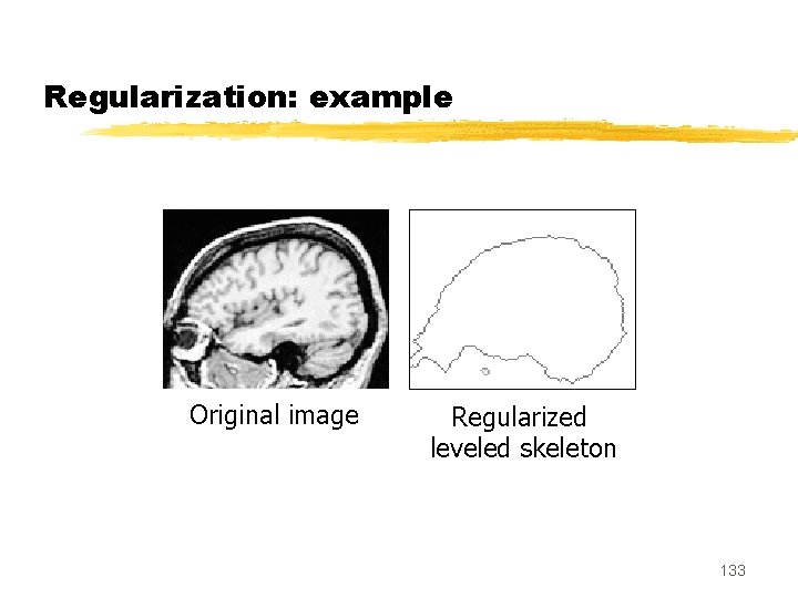
Regularization: example Original image Regularized leveled skeleton 133

Binary reconstruction Original image Regularized skeleton b a 134

Regularization and reconstruction: segmentation without any parameter Original image Regularized leveled skeleton Binary reconstruction 135

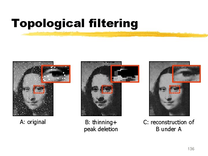
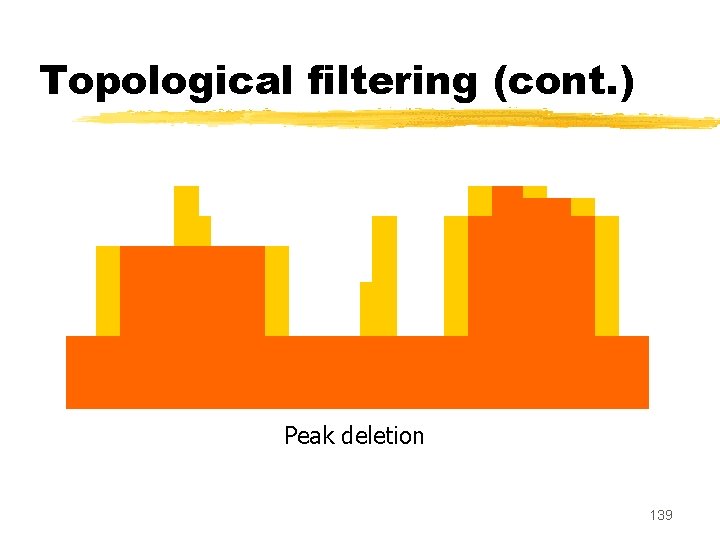
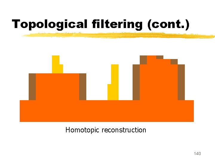
Topological filtering A: original B: thinning+ peak deletion C: reconstruction of B under A 136

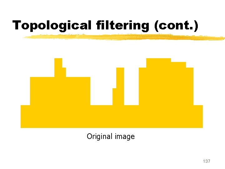
Topological filtering (cont. ) Original image 137

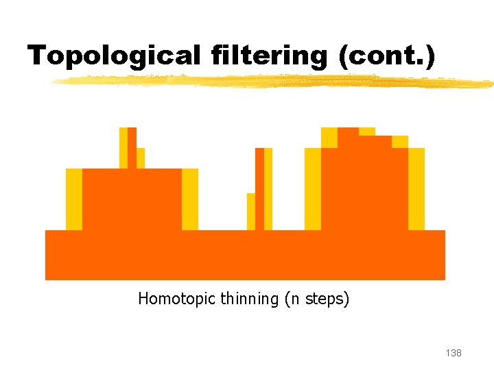
Topological filtering (cont. ) Homotopic thinning (n steps) 138

Topological filtering (cont. ) Peak deletion 139

Topological filtering (cont. ) Homotopic reconstruction 140

Topological filtering (cont. ) Final result 141

Comparison with the morphological approach z. Morphological opening (erosion, dilation): makes no difference between a disk of diameter d an elongated object of thickness d. z. Area opening: makes no difference between a disk and an elongated object having the same area 142

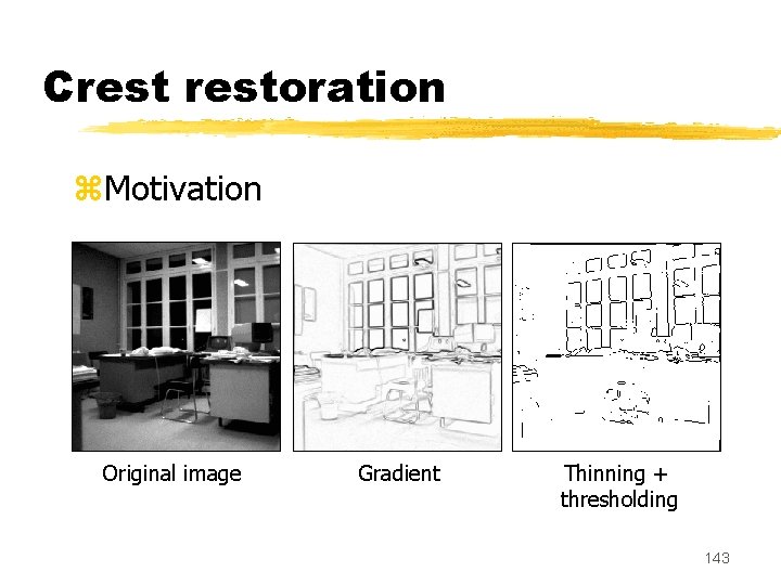
Crestoration z. Motivation Original image Gradient Thinning + thresholding 143

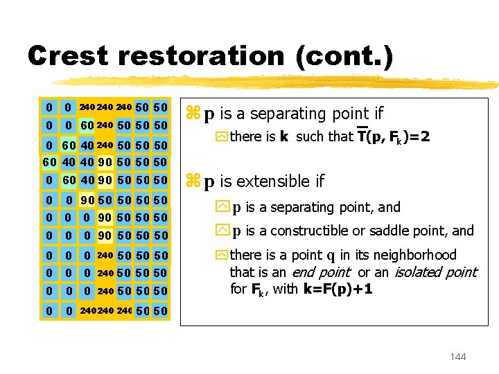
Crestoration (cont. ) 0 0 60 240 50 50 50 240 240 50 50 0 60 40 240 50 50 50 60 40 40 90 50 50 50 0 60 40 90 50 50 50 0 0 90 50 50 50 0 0 0 240 50 50 50 0 90 50 50 50 240 240 z p is a separating point if y there is k such that T(p, Fk)=2 z p is extensible if yp is a separating point, and yp is a constructible or saddle point, and y there is a point q in its neighborhood that is an end point or an isolated point for Fk, with k=F(p)+1 50 50 144

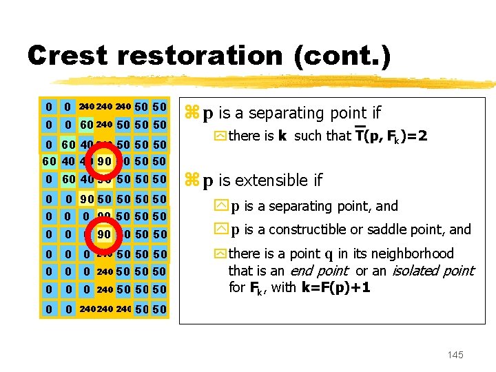
Crestoration (cont. ) 0 0 60 240 50 50 50 240 240 50 50 0 60 40 240 50 50 50 60 40 40 90 50 50 50 0 60 40 90 50 50 50 0 0 90 50 50 50 0 0 0 240 50 50 50 0 90 50 50 50 240 240 z p is a separating point if y there is k such that T(p, Fk)=2 z p is extensible if yp is a separating point, and yp is a constructible or saddle point, and y there is a point q in its neighborhood that is an end point or an isolated point for Fk, with k=F(p)+1 50 50 145

Crestoration (cont. ) 0 0 0 240 240 240 50 50 0 60 240 50 50 50 0 0 0 240 240 50 50 0 60 240 50 50 50 0 60 40 240 50 50 50 60 40 40 240 50 50 50 0 60 40 90 50 50 50 0 60 40240 50 50 50 0 0 90 50 50 50 0 90 50 50 0 240 50 50 50 0 60 40 240 50 50 50 0 240 50 50 50 0 0 0 240 50 50 50 0 0 240 50 50 50 0 0 0 0 240 50 50 50 0 240 50 50 50 0 0 240 240 240 50 50 146

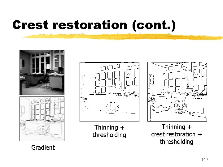
Crestoration (cont. ) Thinning + thresholding Gradient Thinning + crestoration + thresholding 147

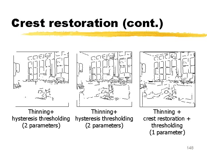
Crestoration (cont. ) Thinning+ hysteresis thresholding (2 parameters) Thinning + crestoration + thresholding (1 parameter) 148

149

Crest Restoration: result ‘Significant’ crests have been highlighted (in green) Before crestoration: After crestoration: 150

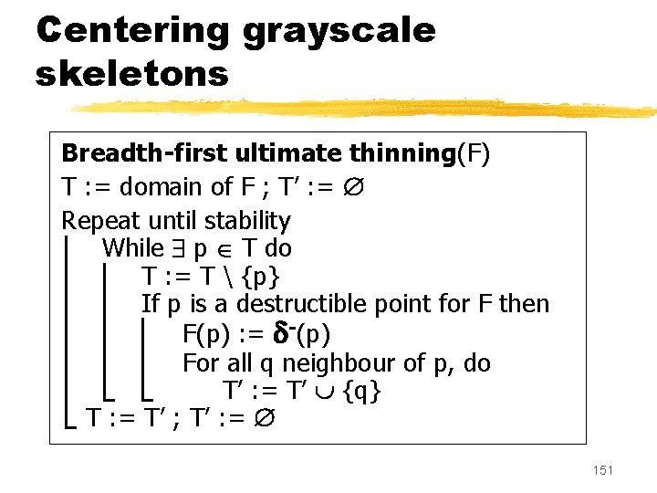
Centering grayscale skeletons Breadth-first ultimate thinning(F) T : = domain of F ; T’ : = Repeat until stability While p T do T : = T {p} If p is a destructible point for F then F(p) : = -(p) For all q neighbour of p, do T’ : = T’ {q} T : = T’ ; T’ : = 151

Breadth-first ultimate thinning : example 152

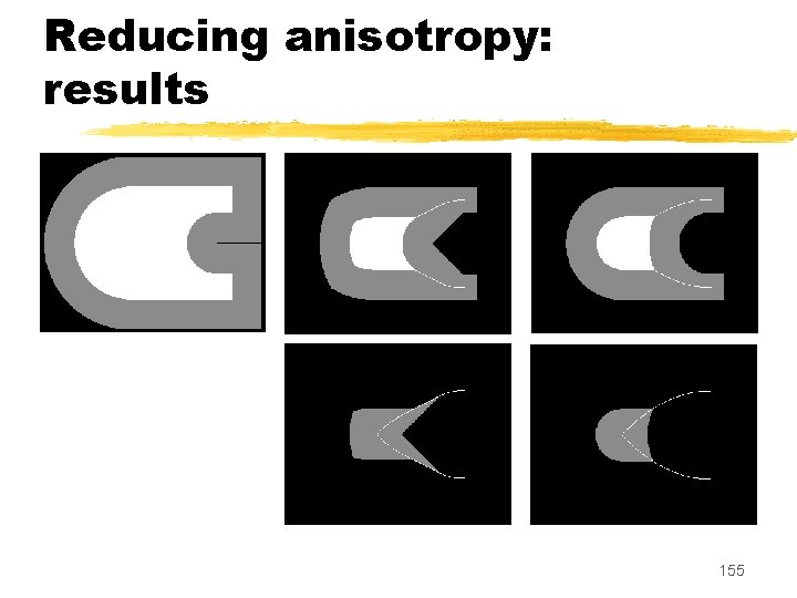
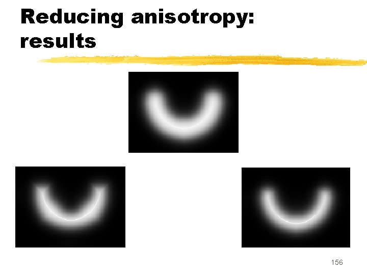
New strategies to reduce anisotropy z. Generalized Euclidean distance map (computes one distance map for each cross-section) z. Dynamic estimation of Euclidean distance (uses the Danielson’s principle and approximation) 153

Reducing anisotropy: results 154

Reducing anisotropy: results 155

Reducing anisotropy: results 156

Conclusion (2 nd part) z. Strict preservation of both topological and grayscale information z. Combining topology-preserving and topology-altering operators z. Control based on several criteria (contrast, size, topology) z. Strategies to reduce anisotropy 157

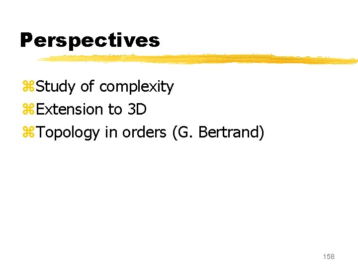
Perspectives z. Study of complexity z. Extension to 3 D z. Topology in orders (G. Bertrand) 158

Perspectives z G. Bertrand, J. C. Everat and M. Couprie: "Image segmentation through operators based upon topology", Journal of Electronic Imaging, Vol. 6, No. 4, pp. 395 -405, 1997. z M. Couprie, F. N. Bezerra, Gilles Bertrand: "Topological operators for grayscale image processing", Journal of Electronic Imaging, Vol. 10, No. 4, pp. 1003 -1015, 2001. z www. esiee. fr/~coupriem/Sdi/publis. html 159