Digital Processing of Speech Signals Static Analysis7 Neural

Digital Processing of Speech Signals Static Analysis(7) Neural Networks Dong Wang CSLT, Tsinghua University 2017. 04 Adopted from Peter Andras: Artificial Neural Network- Introduction peter. andras@ncl. ac. uk

Overview 1. Biological inspiration 2. Artificial neurons and neural networks 3. Learning processes 4. Applications

Biological inspiration l Animals are able to react adaptively to changes in their external and internal environment ü Actually, our brain is not very different from pigs …. ü No special materials were found in brain of smart people ü No special materials were found in high-ability function areas ü If fail to stand up due to a crash, don’t worry, you still have the chance l There must be some thing special different from ‘material’ in the brain that determines its power!

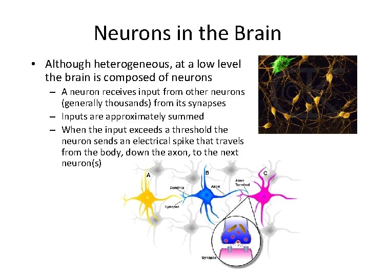
Neurons in the Brain • Although heterogeneous, at a low level the brain is composed of neurons – A neuron receives input from other neurons (generally thousands) from its synapses – Inputs are approximately summed – When the input exceeds a threshold the neuron sends an electrical spike that travels from the body, down the axon, to the next neuron(s)

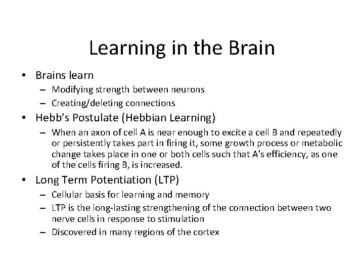
Learning in the Brain • Brains learn – Modifying strength between neurons – Creating/deleting connections • Hebb’s Postulate (Hebbian Learning) – When an axon of cell A is near enough to excite a cell B and repeatedly or persistently takes part in firing it, some growth process or metabolic change takes place in one or both cells such that A's efficiency, as one of the cells firing B, is increased. • Long Term Potentiation (LTP) – Cellular basis for learning and memory – LTP is the long-lasting strengthening of the connection between two nerve cells in response to stimulation – Discovered in many regions of the cortex

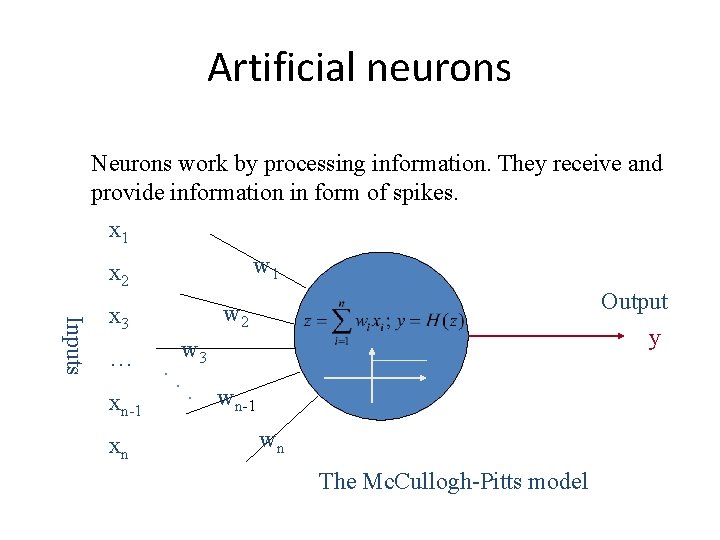
Artificial neurons Neurons work by processing information. They receive and provide information in form of spikes. x 1 w 1 x 2 Inputs … xn-1 xn Output y w 2 x 3. . w 3. wn-1 wn The Mc. Cullogh-Pitts model

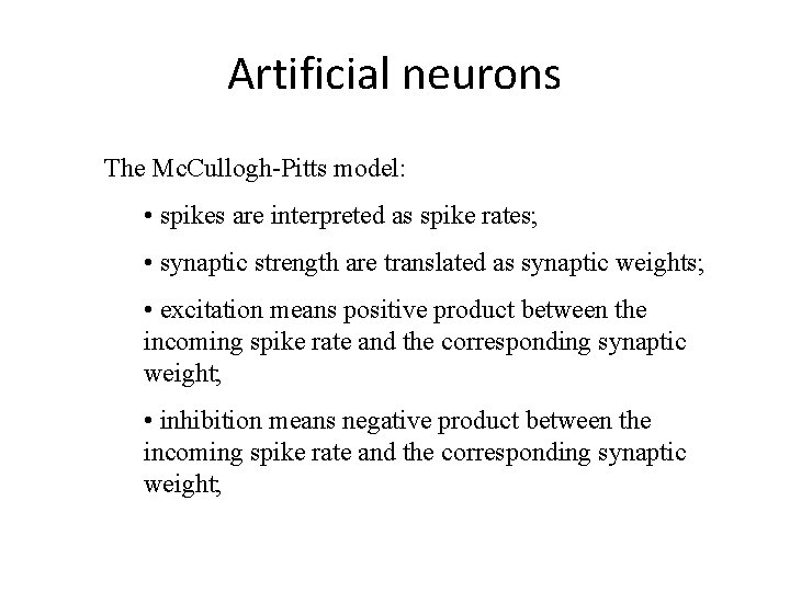
Artificial neurons The Mc. Cullogh-Pitts model: • spikes are interpreted as spike rates; • synaptic strength are translated as synaptic weights; • excitation means positive product between the incoming spike rate and the corresponding synaptic weight; • inhibition means negative product between the incoming spike rate and the corresponding synaptic weight;

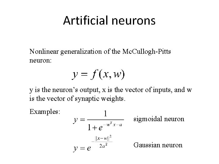
Artificial neurons Nonlinear generalization of the Mc. Cullogh-Pitts neuron: y is the neuron’s output, x is the vector of inputs, and w is the vector of synaptic weights. Examples: sigmoidal neuron Gaussian neuron

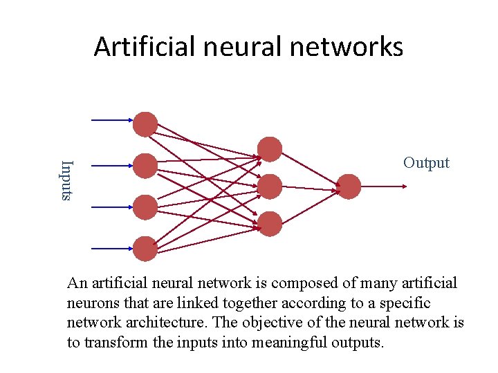
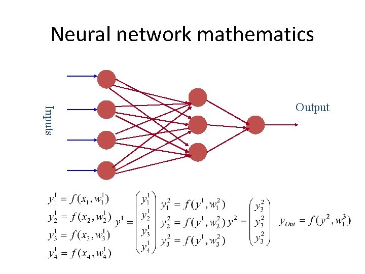
Artificial neural networks Inputs Output An artificial neural network is composed of many artificial neurons that are linked together according to a specific network architecture. The objective of the neural network is to transform the inputs into meaningful outputs.

Artificial neural networks Tasks to be solved by artificial neural networks: • controlling the movements of a robot based on selfperception and other information (e. g. , visual information); • deciding the category of potential food items (e. g. , edible or non-edible) in an artificial world; • recognizing a visual object (e. g. , a familiar face); • predicting where a moving object goes, when a robot wants to catch it.

Learning in biological systems l Learning = learning by adaptation l The young animal learns that the green fruits are sour, while the yellowish/reddish ones are sweet. The learning happens by adapting the fruit picking behavior. l At the neural level the learning happens by changing of the synaptic strengths, eliminating some synapses, and building new ones.

Learning as optimisation l The objective of adapting the responses on the basis of the information received from the environment is to achieve a better state. E. g. , the animal likes to eat many energy rich, juicy fruits that make its stomach full, and makes it feel happy. l In other words, the objective of learning in biological organisms is to optimise the amount of available resources, happiness, or in general to achieve a closer to optimal state.

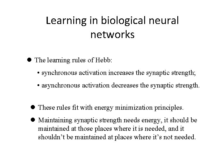
Learning in biological neural networks l The learning rules of Hebb: • synchronous activation increases the synaptic strength; • asynchronous activation decreases the synaptic strength. l These rules fit with energy minimization principles. l Maintaining synaptic strength needs energy, it should be maintained at those places where it is needed, and it shouldn’t be maintained at places where it’s not needed.

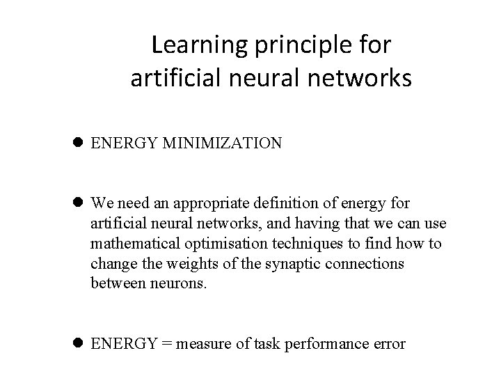
Learning principle for artificial neural networks l ENERGY MINIMIZATION l We need an appropriate definition of energy for artificial neural networks, and having that we can use mathematical optimisation techniques to find how to change the weights of the synaptic connections between neurons. l ENERGY = measure of task performance error

Neural network mathematics Inputs Output

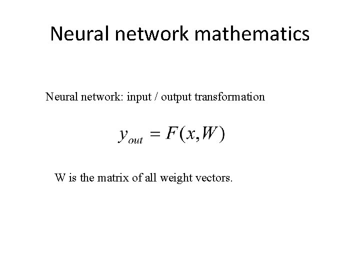
Neural network mathematics Neural network: input / output transformation W is the matrix of all weight vectors.

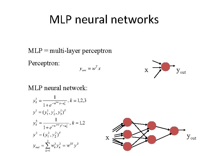
MLP neural networks MLP = multi-layer perceptron Perceptron: x yout MLP neural network: x yout

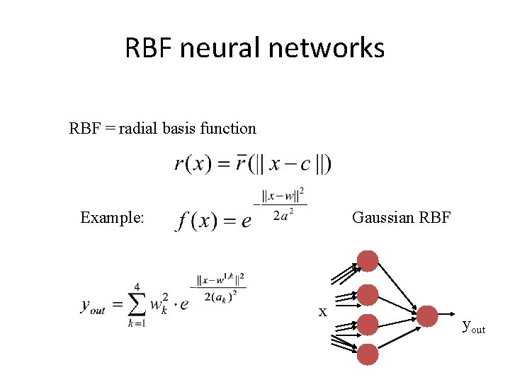
RBF neural networks RBF = radial basis function Example: Gaussian RBF x yout

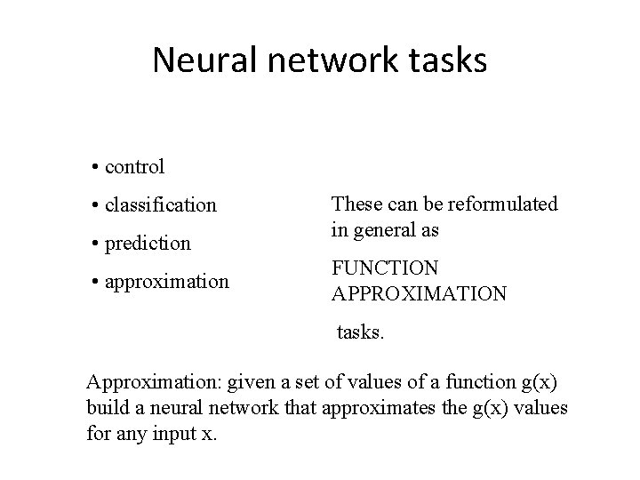
Neural network tasks • control • classification • prediction • approximation These can be reformulated in general as FUNCTION APPROXIMATION tasks. Approximation: given a set of values of a function g(x) build a neural network that approximates the g(x) values for any input x.

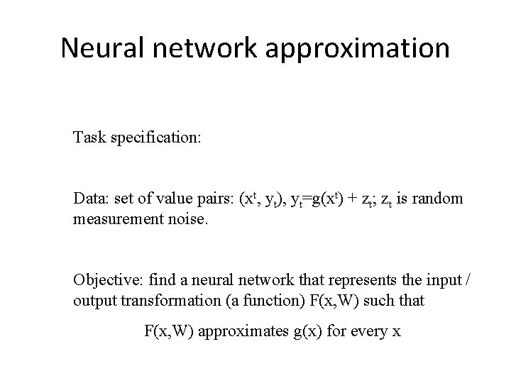
Neural network approximation Task specification: Data: set of value pairs: (xt, yt), yt=g(xt) + zt; zt is random measurement noise. Objective: find a neural network that represents the input / output transformation (a function) F(x, W) such that F(x, W) approximates g(x) for every x

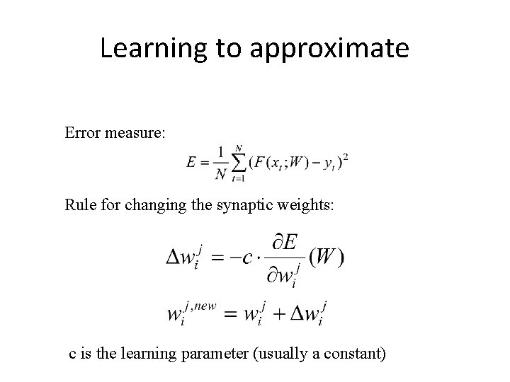
Learning to approximate Error measure: Rule for changing the synaptic weights: c is the learning parameter (usually a constant)

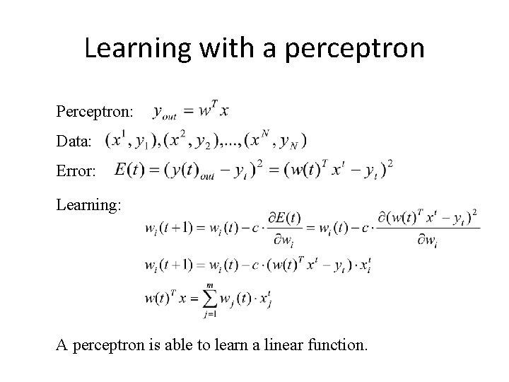
Learning with a perceptron Perceptron: Data: Error: Learning: A perceptron is able to learn a linear function.

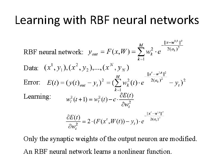
Learning with RBF neural networks RBF neural network: Data: Error: Learning: Only the synaptic weights of the output neuron are modified. An RBF neural network learns a nonlinear function.

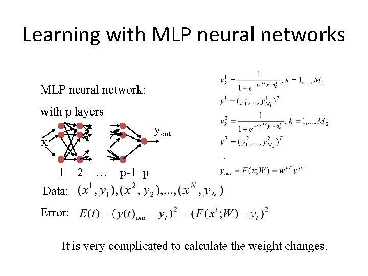
Learning with MLP neural networks MLP neural network: with p layers yout x 1 2 Data: … p-1 p Error: It is very complicated to calculate the weight changes.

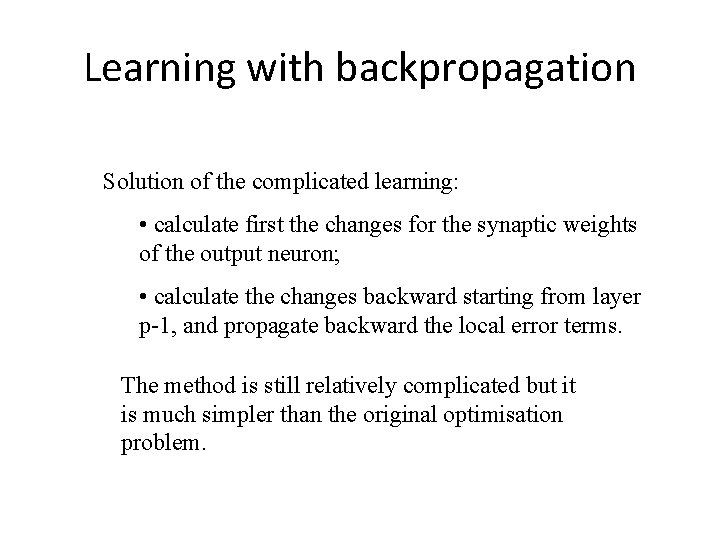
Learning with backpropagation Solution of the complicated learning: • calculate first the changes for the synaptic weights of the output neuron; • calculate the changes backward starting from layer p-1, and propagate backward the local error terms. The method is still relatively complicated but it is much simpler than the original optimisation problem.

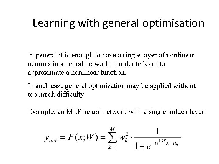
Learning with general optimisation In general it is enough to have a single layer of nonlinear neurons in a neural network in order to learn to approximate a nonlinear function. In such case general optimisation may be applied without too much difficulty. Example: an MLP neural network with a single hidden layer:

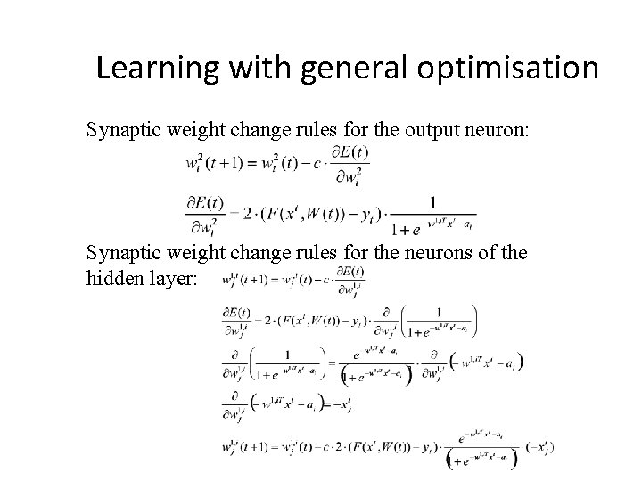
Learning with general optimisation Synaptic weight change rules for the output neuron: Synaptic weight change rules for the neurons of the hidden layer:

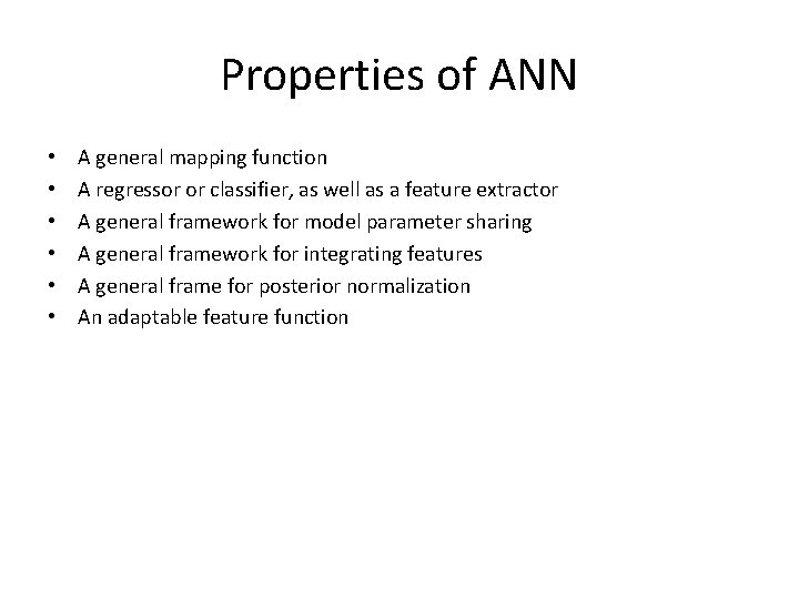
Properties of ANN • • • A general mapping function A regressor or classifier, as well as a feature extractor A general framework for model parameter sharing A general framework for integrating features A general frame for posterior normalization An adaptable feature function

Compare to other models • Compare to linear regression and logistic regression • Compare to probabilistic models (GMM) • Compare to SVM

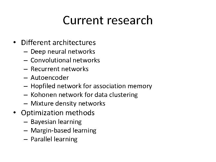
Current research • Different architectures – – – – Deep neural networks Convolutional networks Recurrent networks Autoencoder Hopfiled network for association memory Kohonen network for data clustering Mixture density networks • Optimization methods – Bayesian learning – Margin-based learning – Parallel learning

Current research • Regularization • Adaptation • Multi-task learning

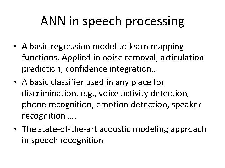
ANN in speech processing • A basic regression model to learn mapping functions. Applied in noise removal, articulation prediction, confidence integration… • A basic classifier used in any place for discrimination, e. g. , voice activity detection, phone recognition, emotion detection, speaker recognition …. • The state-of-the-art acoustic modeling approach in speech recognition

Summary • ANN is a widely used ML model for both regression and classification. • ANN can be interpreted as a feature learning from the input space to a high-dimensional space, layer by layer. It is a learnable feature function. • ANN has a plethora variations, in terms of structure and objective function.

Homework • Use NN to build a speech activity detection system.