Digital Processing of Speech Signals Static Analysis4 EM

Digital Processing of Speech Signals Static Analysis(4) EM Algorithm and Gaussian Mixture Model Dong Wang CSLT, Tsinghua Univ. 2017. 04

Copyright Note: This presentation is partly adopted from the following materials: – Professor Taiwen Yu’s “EM Algorithm”. – Professor Andrew W. Moore’s “Clustering with Gaussian Mixtures”. – Presentation of Haiguang Li, University of Vermont, 2011. 2

Contents 1. 2. 3. 4. Introduction Gaussian mixture model EM-Main Body EM-Algorithm Running on GMM

Model Speech signals with Gaussians • Speech signals can be modeled by Gaussian distributions, but a single Gaussian is probably not enough • Solution: Mixtures of Gaussians

Gaussian mixture model For a single Gaussian, it is simple to estimate the mean and covariance. For a mixture of Gaussians, how to estiamte the parameters?

Starting from Gaussian Sampling

Maximum Likelihood Sampling Given x, it is a function of and 2 We want to maximize it.

Log-Likelihood Function Maximize this instead By setting and

Max. the Log-Likelihood Function

Max. the Log-Likelihood Function

Gaussian Mixture Model (GMM) • Now extend to cluster of Gaussians, or Gaussian mixture model (GMM). .

Gaussian mixture model • The major difficulty of GMM is that we do not know which Gaussian component a training sample belongs to. Or, we miss a variable z that label each sample to its component. • K-mean approach – Assign a sample to its ‘closest’ Gaussian • Soft assignment – Assign a sample to a Gaussian with an associated weight.

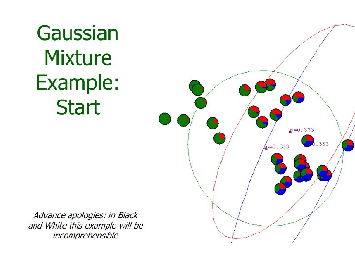
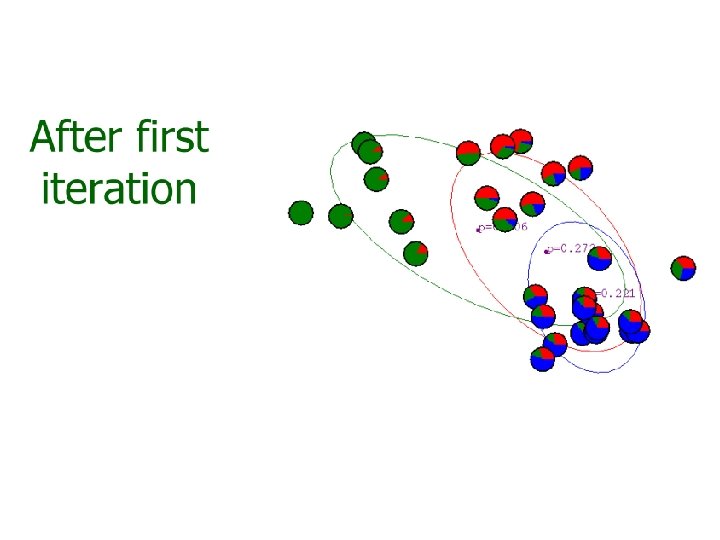
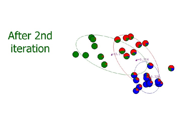
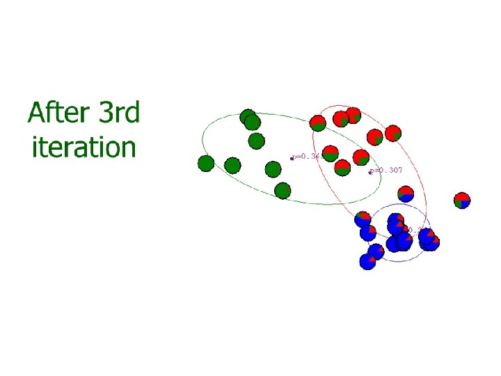
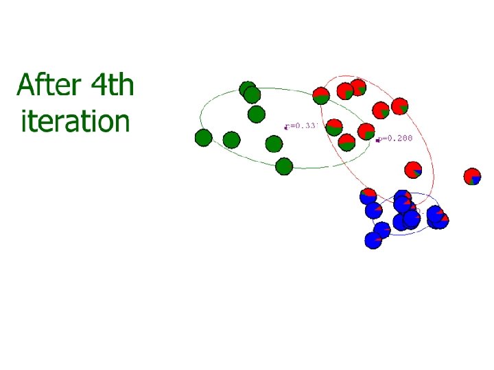
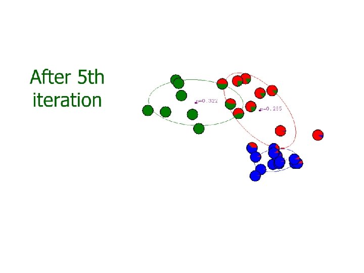
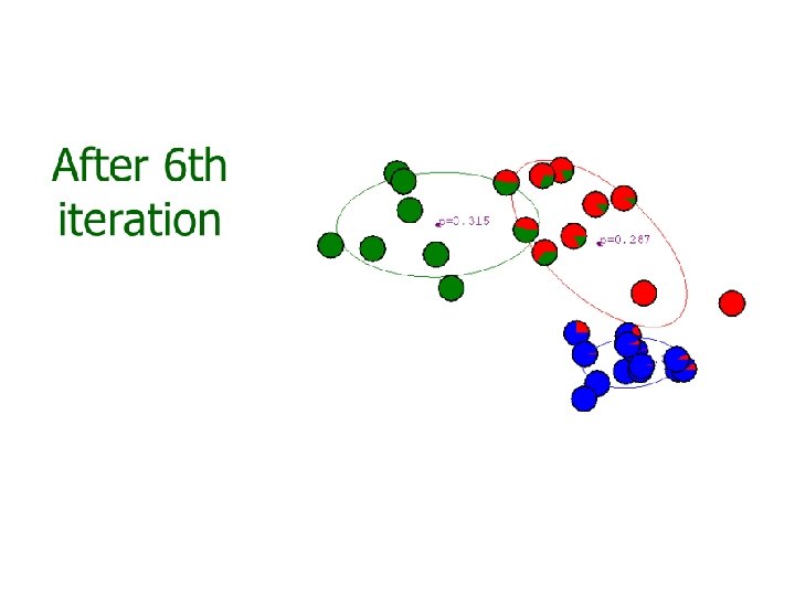
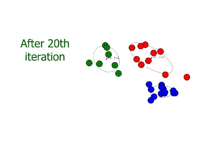
Iterative GMM estimation 1. Initial model parameters: {ϕi, μi, Σi) 2. Compute the soft assignment (weight) of each training sample to each component 3. Optimize model parameters with the soft assignment 4. Repeat (2)-(3) until some criterion reached, e. g. , maximum iterations, small change on parameters

But, we are not sure… • It is really a naïve idea: – If the above process converge? – If the above process find the optimal? – Can and how the above process deal with more complex models? • We hope more mathematical explanatoins

A generative representation • Graphical models φ z μ, Σ x Hidden! N

EM… • We seek a general solution for models with hidden variables {zi}, given observation X. • Iterative estimation with two phases – Estimate the probability of the hidden variable {p(zi|x)} from the visible variables (training data) and the current model parameters – Soft combine the observed variables and the hidden variables according to the probability obtained in the first step to form complete variables. Maximize the model parameters with the complete variable

EM in brief • The EM algorithm was explained and given its name in a classic 1977 paper by Arthur Dempster, Nan Laird, and Donald Rubin. • They pointed out that the method had been "proposed many times in special circumstances" by earlier authors. • EM is typically used to compute maximum likelihood estimates given incomplete samples. • The EM algorithm estimates the parameters of a model iteratively. – Starting from some initial guess, each iteration consists of • an E step (Expectation step) • an M step (Maximization step)

EM Clustering Algorithm

EM Clustering Algorithm (2)

EM for GMM

What’s K-means? • It is a simplified GMM, with hard assignment • The assignment considers only distance, no covariance, i. e. , it assumes shared covariance • It is a special case of EM • E: assignment to clusters • M: estiamte parameters of new clusters (just the mean)

M-step of K-mean

More mathematics This is the EXPECTATION, and we want to maxiize it!

Maximize expectation

Applications • • • Filling in missing data in samples Discovering the value of latent variables Estimating the parameters of HMMs Estimating parameters of finite mixtures Unsupervised learning of clusters …

GMM in speech processing • Speech processing: noise removal, voice activity detection, emotion detection…. • Speech recognition: the former state-of-the -art for acoustic modeling

GMM in speech processing • Speaker recognition: the former state-ofthe-art – GMM-UBM framework • Voice conversion • Speech synthesis: model feature generation

Demos • Matlab demo

Question #1 • What are the main advantages of parametric methods? – You can easily change the model to adapt to different distribution of data sets. – Knowledge representation is very compact. Once the model selected, the model is represented by a specific number of parameters. The number of parameters does not increase with the increasing of training data.

Question #2 • What are the EM algorithm initialization methods? – Random guess. – Initialized by k-means. After a few iterations of k-means, using the parameters to initialize EM.

Question #3 • What are the differences between EM and K-means(or VQ)? – K-means is a simplified EM. – K-means make a hard decision while EM make a soft decision when update the parameters of the model.

Question #4 • How to train a health GMM? – Choose appropriate number of components, Maybe using a development set, or some regulation, such as Bayesian information criterion (BIC). – Choose appropriate structure. Diagonal or full covariance? – Be careful to floor the covariance!

Question 5# • What are the state-of-the-art? – Discriminative training – Bayesian approach – Non-parametric Bayesian approach, such as Dirichlet process GMM (DPGMM)

Question 6# • How GMMs are used in speech processing? – UBM-GMM in speaker recognition – HMM-GMM in speech recognition – HMM-GMM in text to speech – GMM in voice transform

References 1. 2. 3. 4. 5. 6. 7. 8. 9. 10. 11. 12. 13. 14. 15. 16. 17. ^ Dempster, A. P. ; Laird, N. M. ; Rubin, D. B. (1977). "Maximum Likelihood from Incomplete Data via the EM Algorithm". Journal of the Royal Statistical Society. Series B (Methodological) 39 (1): 1– 38. JSTOR 2984875. MR 0501537. ^ Sundberg, Rolf (1974). "Maximum likelihood theory for incomplete data from an exponential family". Scandinavian Journal of Statistics 1 (2): 49– 58. JSTOR 4615553. MR 381110. ^ a b Rolf Sundberg. 1971. Maximum likelihood theory and applications for distributions generated when observing a function of an exponential family variable. Dissertation, Institute for Mathematical Statistics, Stockholm University. ^ a b Sundberg, Rolf (1976). "An iterative method for solution of the likelihood equations for incomplete data from exponential families". Communications in Statistics – Simulation and Computation 5 (1): 55– 64. doi: 10. 1080/03610917608812007. MR 443190. ^ See the acknowledgement by Dempster, Laird and Rubin on pages 3, 5 and 11. ^ G. Kulldorff. 1961. Contributions to theory of estimation from grouped and partially grouped samples. Almqvist & Wiksell. ^ a b Anders Martin-Löf. 1963. "Utvärdering av livslängder i subnanosekundsområdet" ("Evaluation of sub-nanosecond lifetimes"). ("Sundberg formula") ^ a b Per Martin-Löf. 1966. Statistics from the point of view of statistical mechanics. Lecture notes, Mathematical Institute, Aarhus University. ("Sundberg formula" credited to Anders Martin-Löf). ^ a b Per Martin-Löf. 1970. Statistika Modeller (Statistical Models): Anteckningar från seminarier läsåret 1969– 1970 (Notes from seminars in the academic year 1969 -1970), with the assistance of Rolf Sundberg. Stockholm University. ("Sundberg formula") ^ a b Martin-Löf, P. The notion of redundancy and its use as a quantitative measure of the deviation between a statistical hypothesis and a set of observational data. With a discussion by F. Abildgård, A. P. Dempster, D. Basu, D. R. Cox, A. W. F. Edwards, D. A. Sprott, G. A. Barnard, O. Barndorff-Nielsen, J. D. Kalbfleisch and G. Rasch and a reply by the author. Proceedings of Conference on Foundational Questions in Statistical Inference (Aarhus, 1973), pp. 1– 42. Memoirs, No. 1, Dept. Theoret. Statist. , Inst. Math. , Univ. Aarhus, 1974. ^ a b Martin-Löf, Per The notion of redundancy and its use as a quantitative measure of the discrepancy between a statistical hypothesis and a set of observational data. Scand. J. Statist. 1 (1974), no. 1, 3– 18. ^ Wu, C. F. Jeff (Mar. 1983). "On the Convergence Properties of the EM Algorithm". Annals of Statistics 11 (1): 95– 103. doi: 10. 1214/aos/1176346060. JSTOR 2240463. MR 684867. ^ a b Neal, Radford; Hinton, Geoffrey (1999). Michael I. Jordan. ed. "A view of the EM algorithm that justifies incremental, sparse, and other variants". Learning in Graphical Models (Cambridge, MA: MIT Press): 355– 368. ISBN 0262600323. Retrieved 2009 -03 -22. ^ a b Hastie, Trevor; Tibshirani, Robert; Friedman, Jerome (2001). "8. 5 The EM algorithm". The Elements of Statistical Learning. New York: Springer. pp. 236– 243. ISBN 0 -387 -95284 -5. ^ Jamshidian, Mortaza; Jennrich, Robert I. (1997). "Acceleration of the EM Algorithm by using Quasi-Newton Methods". Journal of the Royal Statistical Society: Series B (Statistical Methodology) 59 (2): 569– 587. doi: 10. 1111/1467 -9868. 00083. MR 1452026. ^ Meng, Xiao-Li; Rubin, Donald B. (1993). "Maximum likelihood estimation via the ECM algorithm: A general framework". Biometrika 80 (2): 267– 278. doi: 10. 1093/biomet/80. 2. 267. MR 1243503. ^ Hunter DR and Lange K (2004), A Tutorial on MM Algorithms, The American Statistician, 58: 30 -37