DIGITAL IMAGE Typically composed of picture elements pixels

DIGITAL IMAGE Typically composed of picture elements (pixels) located at the intersection of each row i and column j in each K bands of imagery. Each pixel has some Digital Number (DN) or Brightness Value (BV), that depicts the average radiance of a relatively small area within a scene. A smaller number indicates low average radiance from the area and the high number is an indicator of high radiant properties of the area. As pixel size is reduced more scene detail is presented in digital representation.

Image Rectification a & b Input and reference image with GCP locations, (c) using polynomial equations the grids are fitted together, (d) using resampling method the output grid pixel values are assigned

IMAGE ENHANCEMENT TECHNIQUES Improve the quality of an image as perceived by a human Most useful because many satellite images when examined on a colour display give inadequate information for image interpretation. Image enhancement is attempted after the image is corrected for geometric and radiometric distortions. Image enhancement methods are applied separately to each band of a multispectral image Variety of techniques for improving image quality, i. e. contrast stretch, density slicing, edge enhancement, and spatial filtering are the more commonly used techniques. Digital techniques have been found to be most satisfactory than the photographic technique for image enhancement, because of the precision and wide variety of digital processes.

Contrast Refers to the difference in luminance or grey level values in an image and is an important characteristic. As the ratio of the maximum intensity to the minimum intensity over an image. Contrast ratio has a strong bearing on the resolving power and detectability of an image. Larger this ratio, easier to interpret the image. Satellite images lack adequate contrast and require contrast improvement. Contrast Enhancement To expand the range of brightness values in an image so that the image can be efficiently displayed in a manner desired by the analyst. The density values in a scene are literally pulled farther apart, that is, expanded over a greater range. The effect is to increase the visual contrast between two areas of different uniform densities. This enables the analyst to discriminate easily between areas initially having a small difference in density.

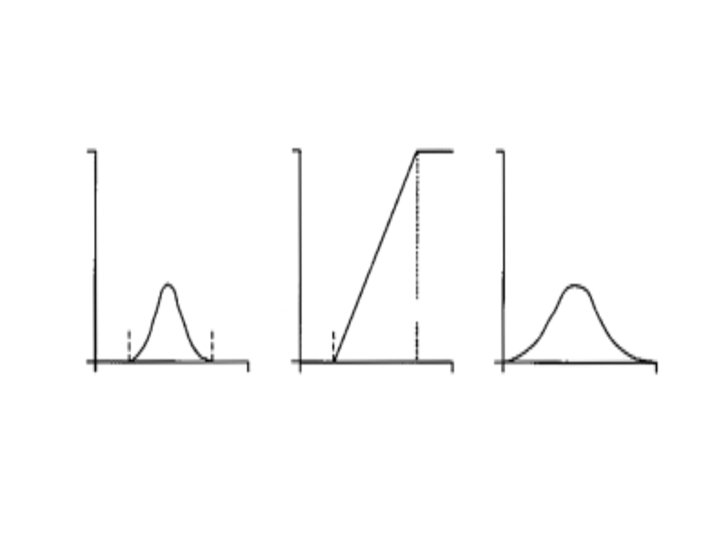
Linear Contrast Stretch Simplest contrast stretch algorithm grey values in the original image and the modified image follow a linear relation in this algorithm. A density number in the low range of the original histogram is assigned to extremely black and a value at the high end is assigned to extremely white. The remaining pixel values are distributed linearly between these extremes. The features or details that were obscure on the original image will be clear in the contrast stretched image. To provide optimal contrast and colour variation in colour composites the small range of grey values in each band is stretched to the full brightness range of the output or display unit.

Non-Linear Contrast Enhancement The input and output data values follow a non-linear transformation. The general form of the non-linear contrast enhancement is defined by y = f (x), where x is the input data value and y is the output data value. Useful for enhancing the colour contrast between the nearly classes and subclasses of a main class. A type of non linear contrast stretch involves scaling the input data logarithmically. This enhancement has greatest impact on the brightness values found in the darker part of histogram. It could be reversed to enhance values in brighter part of histogram by scaling the input data using an inverse log function. Histogram equalization is another non-linear contrast enhancement technique. histogram of the original image is redistributed to produce a uniform population density. This is obtained by grouping certain adjacent grey values. Thus the number of grey levels in the enhanced image is less than the number of grey levels in the original image.

SPATIAL FILTERING A characteristic of remotely sensed images is a parameter called spatial frequency defined as number of changes in Brightness Value per unit distance for any particular part of an image. If there are very few changes in Brightness Value once a given area in an image, this is referred to as low frequency area. Conversely, if the Brightness Value changes dramatically over short distances, this is an area of high frequency. Process of dividing the image into its constituent spatial frequencies, and selectively altering certain spatial frequencies to emphasize some image features. This technique increases the analyst’s ability to discriminate detail. The three types of spatial filters used in remote sensor data processing are : Low pass filters, Band pass filters and High pass filters.

Low-Frequency Filtering in the Spatial Domain Image enhancements that de-emphasize or block the high spatial frequency detail are low-frequency or low-pass filters. Low-frequency filter evaluates a particular input pixel brightness value, BVin, and the pixels surrounding the input pixel, and outputs a new brightness value, BVout , that is the mean of this convolution. The size of the neighbourhood convolution mask or kernel (n) is usually 3 x 3, 5 x 5, 7 x 7, or 9 x 9. The simple smoothing operation will, however, blur the image, especially at the edges of objects. Blurring becomes more severe as the size of the kernel increases. Using a 3 x 3 kernel can result in the low-pass image being two lines and two columns smaller than the original image. Techniques that can be applied to deal with this problem include (1) artificially extending the original image beyond its border by repeating the original border pixel brightness values or (2) replicating the averaged brightness values near the borders, based on the image behaviour within a view pixels of the border. The most commonly used low pass filters are mean, median and mode filters.

High-Frequency Filtering in the Spatial Domain Applied to imagery to remove the slowly varying components and enhance the high-frequency local variations. Enhances higher frequencies, suppress lower ones. Brightness values tend to be highly correlated in a nineelement window. Hence, the high frequency filtered image will have a relatively narrow intensity histogram. This suggests that the output from most high-frequency filtered images must be contrast stretched prior to visual analysis.

Edge Enhancement in the Spatial Domain For many remote sensing earth science applications, the most valuable information that may be derived from an image is contained in the edges surrounding various objects of interest. Edge enhancement delineates these edges and makes the shapes and details comprising the image more conspicuous and perhaps easier to analyze. Generally, what we see as pictorial edges are simply sharp changes in brightness value between two adjacent pixels. The edges may be enhanced using either linear or nonlinear edge enhancement techniques.

Linear Edge Enhancement A straightforward method of extracting edges in remotely sensed imagery is the application of a directional firstdifference algorithm and approximates the first derivative between two adjacent pixels. The algorithm produces the first difference of the image input in the horizontal, vertical, and diagonal directions. The Laplacian operator generally highlights point, lines, and edges in the image and suppresses uniform and smoothly varying regions. Human vision physiological research suggests that we see objects in much the same way. Hence, the use of this operation has a more natural look than many of the other edge-enhanced images.

Band ratioing Sometimes differences in brightness values from identical surface materials are caused by topographic slope and aspect, shadows, or seasonal changes in sunlight illumination angle and intensity. May hamper the ability of an interpreter or classification algorithm to identify correctly surface materials or land use in a remotely sensed image. Fortunately, ratio transformations of the remotely sensed data can, in certain instances, be applied to reduce the effects of such environmental conditions. In addition to minimizing the effects of environmental factors, ratios may also provide unique information not available in any single band that is useful for discriminating between soils and vegetation.

The mathematical expression of the ratio function is BVi, j, r = BVi, j, k/BVi, j. l where BVi, j, r is the output ratio value for the pixel at row, i, column j; BVi, j, k is the brightness value at the same location in band k, and BVi, j, l is the brightness value in band l. However, the computation is not always simple since BVi, j = 0 is possible. But, there alternatives. For example, the mathematical domain of the function is 1/255 to 255 (i. e. , the range of the ratio function includes all values beginning at 1/255, passing through 0 and ending at 255). The way to overcome this problem is simply to give any BVi, j with a value of 0 the value of 1.

Ratio images can be meaningfully interpreted because they can be directly related to the spectral properties of materials. Ratioing can be thought of as a method of enhancing minor differences between materials by defining the slope of spectral curve between two bands. dissimilar materials having similar spectral slopes but different albedos, which are easily separable on a standard image, may become inseparable on ratio images. e. g. Deciduous and Coniferous Vegetation crops out on both the sunlit and shadowed sides of a ridge. In the individual bands the reflectance values are lower in the shadowed area and it would be difficult to match this outcrop with the sunlit outcrop. The ratio values, however, are nearly identical in the shadowed and sunlit areas and the sandstone outcrops would have similar signatures on ratio images. This removal of illumination differences also eliminates the dependence of topography on ratio images.

Land cover/Illumination Digital No. Ratio Band A Band B ______________________________ Deciduous Sun lit 48 50 0. 96 Shadow 18 19 0. 95 Coniferous Sunlit 31 45 0. 69 Shadow 11 16 0. 69 ______________________________