Digital Image Processing Using MATLAB Wild Cat http

Digital Image Processing Using MATLAB® Wild Cat • http: //www. youtube. com/watch? v=w. E 3 fm. FTt P 9 g&feature=player_embedded
의 3 3 이웃")
Digital Image Processing Using MATLAB® 그림 3. 1 (x, y)의 3 3 이웃

Digital Image Processing Using MATLAB®

Digital Image Processing Using MATLAB®

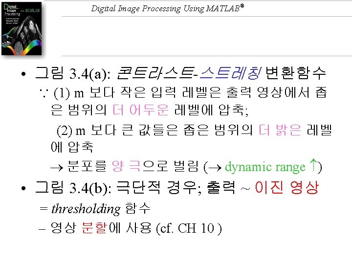
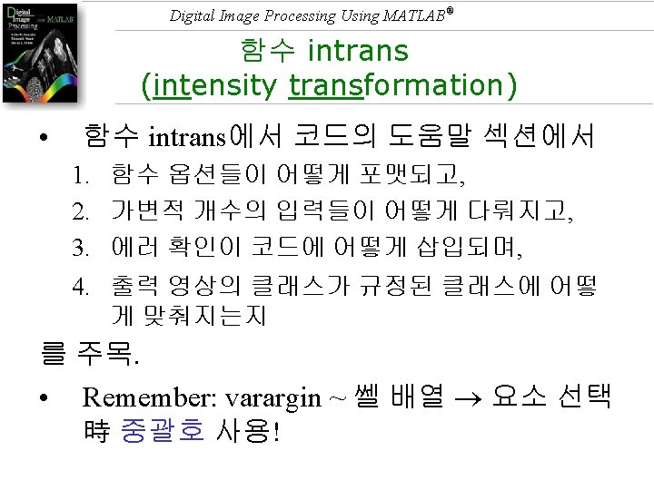
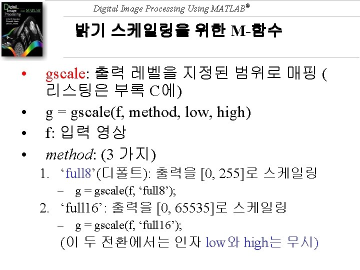
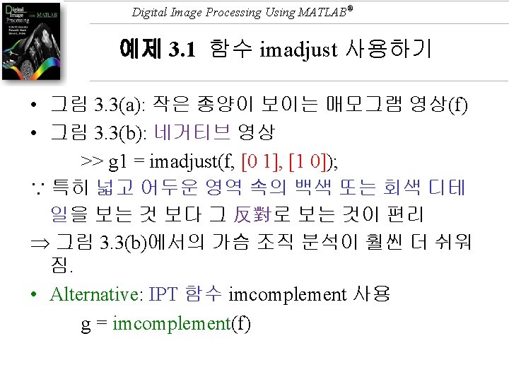
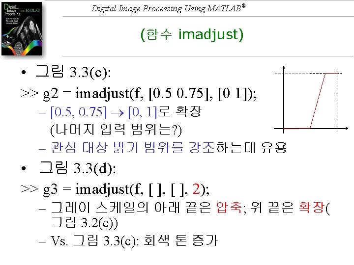
Digital Image Processing Using MATLAB® 3. 2. 1 함수 imadjust • 그레이 영상의 밝기 변환을 위한 기본적인 IPT 툴: g = imadjust(f, [low_in high_in], [low_out high_out], gamma) • [low_in, high_in] [low_out, high_out] • clipping: (그림 3. 2)
 • Linear scaling – Replace the")
Digital Image Processing Using MATLAB® Histogram modification (2) • Linear scaling – Replace the gray value of by. – The resulting histogram has gaps between bins. Figure 4. 2, pg 114

Digital Image Processing Using MATLAB®
")
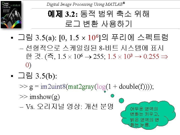
Digital Image Processing Using MATLAB® 2차원 스펙트럼 그림 3. 5(a)

Digital Image Processing Using MATLAB®
. .")
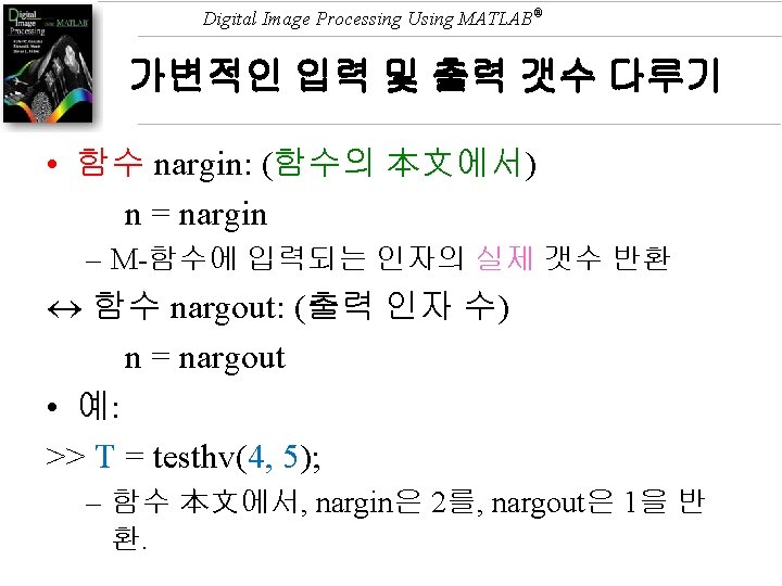
Digital Image Processing Using MATLAB® 보기 function G = testhv 2(x, y, z). . . error(nargchk(2, 3, nargin)); . . . • 예: >> testhv 2(6); % nargin == 1 Not enough input arguments. • and 실행 중단.

Digital Image Processing Using MATLAB® 변수 varargin과 varargout • 변수 varargin과 varargout ~소문자 • 예: function [m, n] = testhv 3(varargin) 입력 인자 수 ~ 可變的 function [varargout] = testhv 4(m, n, p) 출력 인자 수 ~ 가변적

Digital Image Processing Using MATLAB® 예제 3. 4: 영상 히스토그램을 계산하 고 그리기 그림 3. 3(a)(영상 f) imhist(f) 그림 3. 7(a)
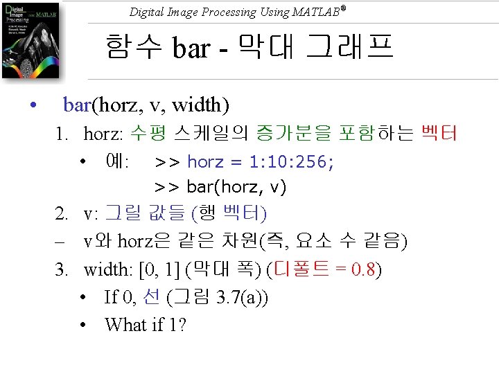

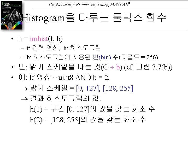
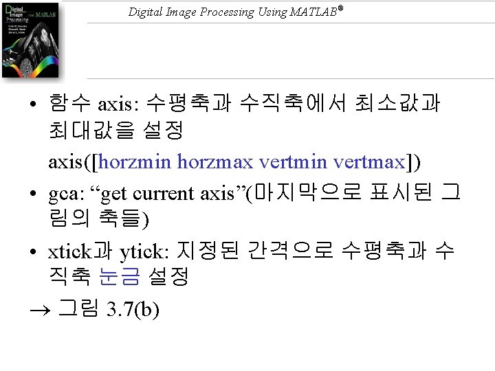
Digital Image Processing Using MATLAB® 함수 bar 연습 • 수평축을 10 개의 레벨의 그룹들로 나누어 막대 그 래프 만들기: >> f = imread('Fig 0303(a)(breast). tif'); >> h = imhist(f); % histogram 값 계산 >> v = h(1: 10: 256); % 10 개씩 묶어서 다시 계산 >> horz = 1: 10: 256; % 플롯할 값의 수와 빈 수를 맞춰줌 >> bar(horz, v) >> axis([0 255 0 15000]) >> set(gca, ‘xtick’, 0: 50: 255) >> set(gca, ‘ytick’, 0: 2000: 15000)

Digital Image Processing Using MATLAB®
 ?")
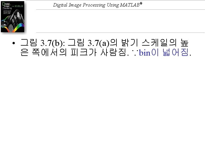
Digital Image Processing Using MATLAB® • 그림 3. 7(b) ?
에")
Digital Image Processing Using MATLAB® If horz is omitted 수평 축의 bin 폭을 length(v)에 의해 결정: (Why? Ans) 同차원) >> bar(v) >> axis([0 26 0 15000])

Digital Image Processing Using MATLAB® 기타 그래프 축 설정 함수들 • axis labels: xlabel(‘text string’, ‘fontsize’, size) – size: font size in points • Text to the body of the figure: text(xloc, yloc, ‘text string’, ‘fontsize’, size) (예제: 3. 5 ) • 注: Functions that set axis values and labels are used after the function has been plotted.
 – centered above the plot")
Digital Image Processing Using MATLAB® • title(‘titlestring’) – centered above the plot
 (그림 3. 7(c)) stem(horz,")
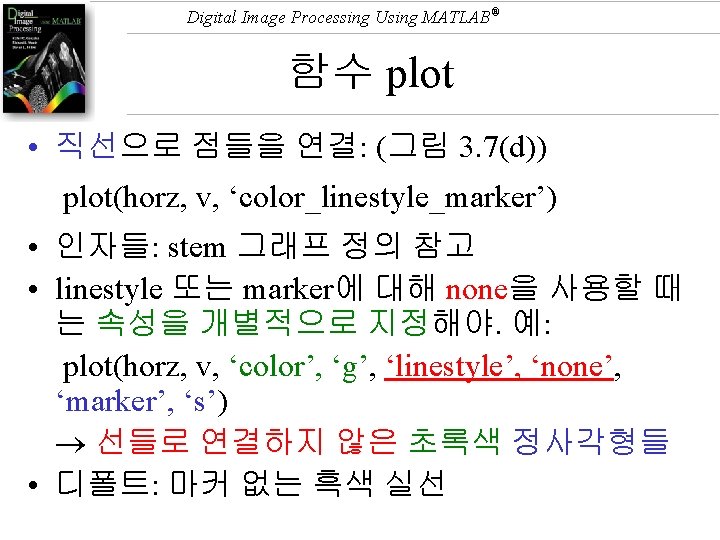
Digital Image Processing Using MATLAB® stem 그래프 (막대 그래프와 비슷) (그림 3. 7(c)) stem(horz, v, ‘color_linestyle_marker’, ‘fill’) horz, v: bar 참고 color_linestyle_marker: 3중 값 from 표 3. 1 예: stem(v, ‘r--s') 선과 마커가 붉고(red), 선은 파선(dashed)이고, 마커는 정사각형 (square)

Digital Image Processing Using MATLAB® 함수 stem과 plot의 속성들 함수 stem과 plot에 대한 추가 옵션은 stem 도움말 페이지를 참고
 fill이 사용되고,")
Digital Image Processing Using MATLAB® stem – ‘fill’ 인자 • If (1) fill이 사용되고, (2) 마커가 원, 정사각형, or 다이아몬드, 마커를 color에 지정된 칼라로 채움. • 디폴트: 칼라 = black, 선 = solid, 마커 = circle • 그림 3. 7(c): (stem 그래프) >> h = imhist(f); v = h(1: 10: 256); horz = 1: 10: 256; >> stem(horz, v, ‘fill’) >> axis([0 255 0 15000]) >> set(gca, ‘xtick’, [0: 50: 255]) >> set(gca, ‘ytick’, [0: 2000: 15000))
 >> h = imhist(f); >> plot(h)")
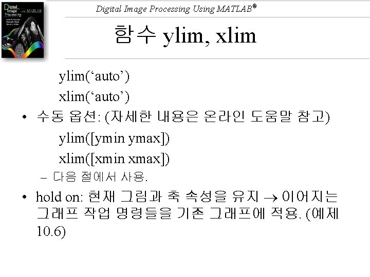
Digital Image Processing Using MATLAB® 그림 3. 7(d) >> h = imhist(f); >> plot(h) % Use the default values >> axis([0 255 0 15000]) >> set(gca, ‘xtick’, [0: 50: 255]) >> set(gca, ‘ytick’, [0: 2000: 15000)) • 함수 plot 사용 예: 그림 2. 6(e), 그림 3. 9 (예 제 3. 5) • 축 한계와 눈금 표시를 자동으로 설정 가능: (함수 ylim, xlim 사용 )

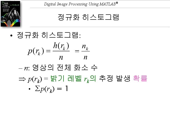
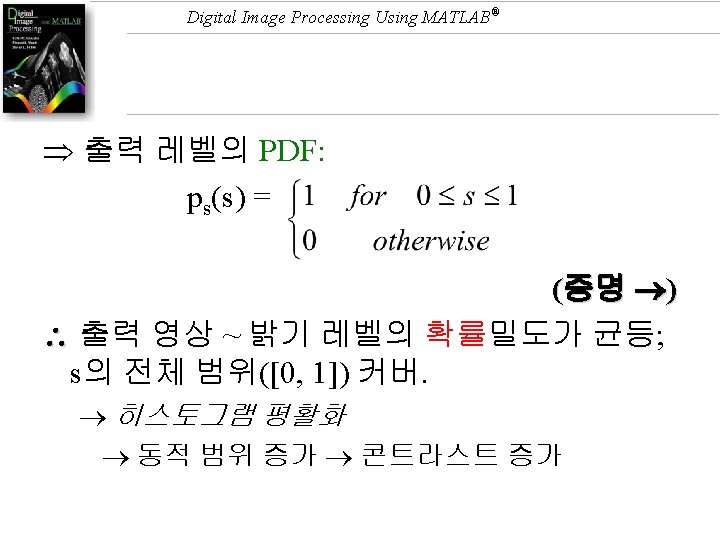
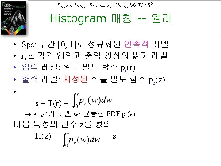
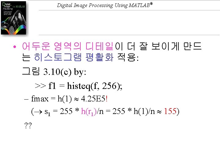
Digital Image Processing Using MATLAB® 3. 3. 2 Histogram 평활화 • 가정: 입력 밝기 레벨 ~ 범위 [0, 1]로 정규화 된 연속적인 값 • pr(r) 영상의 밝기 레벨의 확률 밀도 함수 (probability density function, PDF) (cf. § 3. 3. 1) • 출력 밝기 레벨(= s) 공식: s = T(r) = • 누적 분포 함수(cumulative distribution function, CDF)
 T(r) ~ single-valued, monotonically")
Digital Image Processing Using MATLAB® • 단, two conditions: (a) T(r) ~ single-valued, monotonically increasing in 0 r 1 (b) 0 T(r) 1 for 0 r 1
 = • ds/dr =")
Digital Image Processing Using MATLAB® 증명 • s = T(r) = • ds/dr = d T(r)/dr = pr(r) ( 0 condition (a)) ( ps(s) ds = pr(r) dr) • ps(s) = pr(r) |dr / ds| = pr(r) | 1/ pr(r) | =1 for 0 s 1 (∵ p 0)

Digital Image Processing Using MATLAB® 예제: For a 4 4 image

Digital Image Processing Using MATLAB® 4 4 3 3 7 7 5 5 0 1 2 3 5 (rk) (sk)

Digital Image Processing Using MATLAB® 만일 uint 3가 있다면 sk nk ∑nk 0 2 2 1 2 4 2 2 6 3 6 12 4 4 16 5 0 16 6 0 16 7 0 16 sk = ∑nk / n (uint 3 영상) (= 7) (double 영상) 2/16 = 0. 125 1 0. 250 2 0. 375 3 0. 750 5 1. 000 7
")
Digital Image Processing Using MATLAB® 그림 3. 8 (Histogram 평활화)
 >> imhist(f) (b)")
Digital Image Processing Using MATLAB® 그림 3. 8의 histogram들 그리기 (a) >> imhist(f) (b) 그림 3. 8(b) >> ylim('auto') (c) >> g = histeq(f, 256); >> imhist(g) (d) 그림 3. 8(d) >> ylim('auto')
")
Digital Image Processing Using MATLAB® 변환함수(= cdf)
 그리기 >> hnorm")
Digital Image Processing Using MATLAB® 그림 3. 9의 HE 변환함수(= cdf) 그리기 >> hnorm = imhist(f). /numel(f); >> cdf = cumsum(hnorm); >> x = linspace(0, 1, 256); % 255? >> plot(x, cdf) >> axis([0 1 0 1]) >> set(gca, 'xtick', 0: . 2: 1) >> set(gca, 'ytick', 0: . 2: 1) >> xlabel('Input intensity values', 'fontsize', 9) >> ylabel('Output intensity values', 'fontsize', 9) >> % Specify text in the body of the graph: >> text(0. 18, 0. 5, 'Transformation function', 'fontsize', 9)

Digital Image Processing Using MATLAB® linspace Generate linearly spaced vectors • Syntax: y = linspace(a, b) y = linspace(a, b, n) • similar to the colon operator ": ", but gives direct control over the number of points. • y = linspace(a, b) generates a row vector y of 100 points linearly spaced between and including a and b. • y = linspace(a, b, n) generates a row vector y of n points linearly spaced …

Digital Image Processing Using MATLAB®

Digital Image Processing Using MATLAB® - 인위적…
 %INTRANS Performs intensity (gray-level)")
Digital Image Processing Using MATLAB® function g = intrans(f, varargin) %INTRANS Performs intensity (gray-level) transformations. % G = INTRANS(F, ‘neg’) computes the negative of input image F. %
) % G = INTRANS(F,")
Digital Image Processing Using MATLAB® g = c*log(1 + double(f)) % G = INTRANS(F, ‘log’, C, CLASS) computes log(1 + F) and % multiplies the result by (positive) constant C. If the last two % parameters are omitted, C defaults to 1. Because the log is used frequently to display Fourier spectra, % parameter CLASS offers the % option to specify the class of the output as ‘uint 8’ or % ‘uint 16’. If parameter CLASS is omitted, the output is of the same class as the input. %
 performs a …")
Digital Image Processing Using MATLAB® % G = INTRANS(F, ‘gamma’, GAM) performs a … % % G = INTRANS(F, ‘stretch’, M, E) computes a contraststretching % trasformation using … % % For the

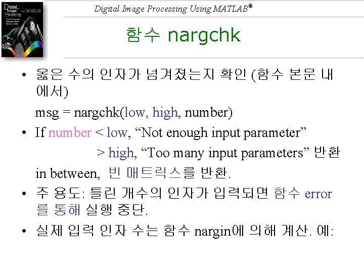
Digital Image Processing Using MATLAB® % Verify the correct number of inputs. error(nargchk(2, 4, nargin)) % nargchk message % classin = class(f); % If the input is of class double, and it is outside the range % [0, 1], and the specified transformation is not ‘log’, convert the % input to the range [0, 1].
, ‘double’) & max(f(: )) > 1 &")
Digital Image Processing Using MATLAB® if strcmp(class(f), ‘double’) & max(f(: )) > 1 & … ~strcmp(varargin{1}, ‘log’) f = mat 2 gray(f); else % Convert to double, … f = im 2 double(f); end % Determine the type of … method = varargin{1};

Digital Image Processing Using MATLAB® neg % Perform the intensity … switch method case ‘neg’ g = imcomplement(f); • switch-case 예: switch (rem(n, 4)==0) + (rem(n, 2)==0) case 0 M = odd_magic(n) case 1 M = single_even_magic(n) case 2 M = double_even_magic(n) otherwise error('This is impossible') end
 == 1 c =")
Digital Image Processing Using MATLAB® log case ‘log’ if length(varargin) == 1 c = 1; elseif length(varargin) == 2 c = varargin{2}; elseif length(varargin) == 3 c = varargin{2}; classout = varargin{3}; else error(‘Incorrect number of inputs for the log option. ’) end g = c*(log(1 + double(f)));
 < 2 error(‘Not enough")
Digital Image Processing Using MATLAB® gamma case ‘gamma’ if length(varargin) < 2 error(‘Not enough inputs for the gamma option. ’) end gam = varargin{2}; g = imadjust(f, [ ], gam);
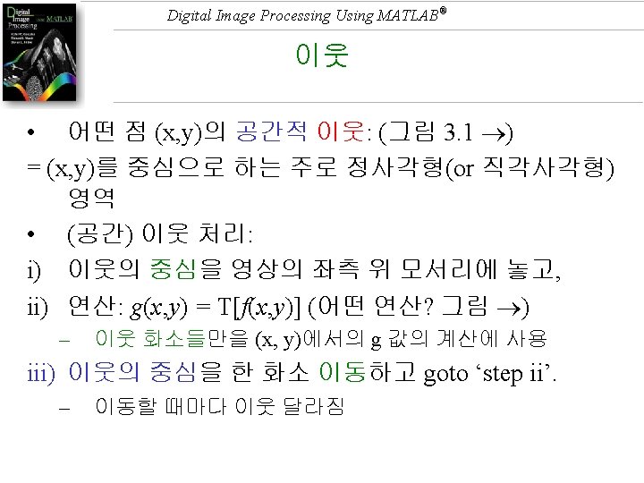
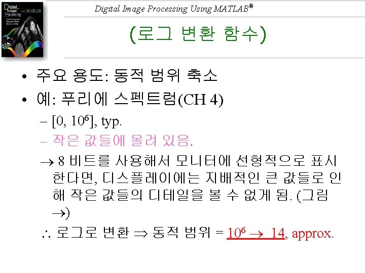
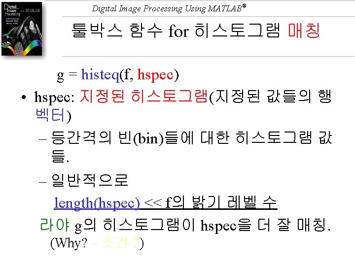
![Digital Image Processing Using MATLAB® imadjust J = imadjust(I, [low_in; high_in], [low_out; high_out], gamma)](http://slidetodoc.com/presentation_image_h/bd48d3479e1628f8553f19811bcb302a/image-77.jpg "Digital Image Processing Using MATLAB® imadjust J = imadjust(I, [low_in; high_in], [low_out; high_out], gamma)")
Digital Image Processing Using MATLAB® imadjust J = imadjust(I, [low_in; high_in], [low_out; high_out], gamma) • gamma < 1 the mapping is weighted toward higher (brighter) output values. • gamma > 1 the mapping is weighted toward lower (darker) output values. • gamma == 1 linear mapping – If you omit the argument, gamma defaults to 1. • If high_out < low_out, the output image is reversed, as in a photographic negative.
 == 1 % Use")
Digital Image Processing Using MATLAB® Contrast-stretching case ‘stretch’ if length(varargin) == 1 % Use defaults. m = mean 2(f); E = 4. 0; elseif length(varargin) == 3 m = varargin{2}; E = varargin{3}; else error(‘Incorrect number of inputs for the stretch option. ’) end g = 1. /(1 + (m. /(f + eps)). ^E);
 end % g =")
Digital Image Processing Using MATLAB® otherwise error(‘Unknown enhancement method. ’) end % g = changeclass(classout, g);

Digital Image Processing Using MATLAB® • mean 2 – Compute the mean of the elements of a matrix

Digital Image Processing Using MATLAB® 예제 3. 3 함수 intrans 사용 하기 • 그림 3. 6(a) 콘트라스트-스트레칭 그림 3. 6(b) >> g = intrans(f, 'stretch', mean 2(im 2 double(f)), 0. 9); – Q 1: Why apply im 2 double? Ans) – Q 2: Why not use mean 2(mat 2 gray(im 2 double(f)))? Ans) >> figure, imshow(g) • 영상 f im 2 double [0. , 1. ]로 스케일링 • 함수 호출 시 f의 평균값 계산(mean 2 사용) • m에 요구되는 대로 평균 또한 이 범위에 듦: (E 값(0. 9)은 대화식으로 결정되었음. )

Digital Image Processing Using MATLAB®
 imhist(f) (b) imhist(im 2 double(f)) (c) intrans(f,")
Digital Image Processing Using MATLAB® histograms (a) imhist(f) (b) imhist(im 2 double(f)) (c) intrans(f, ‘stretch’, mean 2(im 2 double(f)), 0. 9) * mean 2(…) 0. 0672

Digital Image Processing Using MATLAB® • g = 255. * 1. /(1 + (m. /(f + eps)). ^E); where m = 0. 0672 f = 0: (1/256) : 1 E = 0. 9 >> g = 255. * 1. /(1 + (0. 0672. /(f + eps)). ^0. 9);

Digital Image Processing Using MATLAB®
")
Digital Image Processing Using MATLAB® E = 0. 9 (m = 0. 6114)

Digital Image Processing Using MATLAB® >> x = 0: 1/256: 1; >> figure, plot(x, 1. /(1+(m. /(x + eps)). ^E)); % m=. 6114, E=. 9 >> ylim([0 1]) S字?

Digital Image Processing Using MATLAB® M-file로 optimum E 값 찾기 Cell > Evaluate Cell Mode %% if ~isequal(class(gray_im), 'double') f = im 2 double(gray_im); end subplot(2, 2, 1); imshow(f) subplot(2, 2, 3); imhist(f) m = mean 2(f); E = 4. 9; g = 1. /(1 + (m. /(f + eps)). ^E); subplot(2, 2, 2); imshow(g) subplot(2, 2, 4); imhist(g)

Digital Image Processing Using MATLAB® E = 4. 9
). ^E));")
Digital Image Processing Using MATLAB® >> figure, plot(x, 1. /(1+(m. /(x + eps)). ^E));

Digital Image Processing Using MATLAB® g = 255. * 1. /(1 + (m. /(f + eps)). ^E);
 • T(r)의 한계")
Digital Image Processing Using MATLAB® • eps ? (표 2. 10) • T(r)의 한계 값(최대) = 1 출력 값 ~ [0, 1]로 스케일링
)));")
Digital Image Processing Using MATLAB® ! 비교: >> imshow(mat 2 gray(log(1 + double(f))));

Digital Image Processing Using MATLAB® g = im 2 uint 8(mat 2 gray(log(1 + double(f))));

Digital Image Processing Using MATLAB® Photoshop: Image > Adjustment > Curves…
 1. 입력 영상 ~ 클래스 uint 8,")
Digital Image Processing Using MATLAB® (함수 imadjust) 1. 입력 영상 ~ 클래스 uint 8, uint 16, double 형 출력 영상 ~ 입력 영상과 같은 클래스 2. 2 nd & 3 rd 인자 ~ [0, 1] (f의 클래스와 무관) – If f ~ 클래스 uint 8, * 255 If f ~ 클래스 uint 16, * 65535 – If [low_in high_in], [low_out high_out] ~ 빈 매트릭 스([ ]), 디폴트 값 = [0 1] • If high_out < low_out, 출력 밝기 반전

Digital Image Processing Using MATLAB® 밝기 반전 via 대화상자 네거티브 또는, via 메뉴: Image > Adjustment > Invert
 3. gamma: 곡선의 모양을 규정 – If")
Digital Image Processing Using MATLAB® (함수 imadjust) 3. gamma: 곡선의 모양을 규정 – If gamma < 1 (그림 3. 2(a)), 출력 밝기 (Why? ) If gamma > 1, 출력이 어두워져. 만일 생략하면, gamma = 1 (선형 매핑).

Digital Image Processing Using MATLAB®
 vs. (d)")
Digital Image Processing Using MATLAB® 그림 (c) vs. (d)

Digital Image Processing Using MATLAB® histograms

Digital Image Processing Using MATLAB® HE
. /numel(f); >>")
Digital Image Processing Using MATLAB® Cumulative distribution function >> hnorm = imhist(f). /numel(f); >> cdf = cumsum(hnorm); >> plot(cdf) >> ylim([0 1. 01]) >> xlim([0 255])
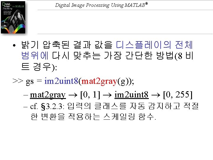
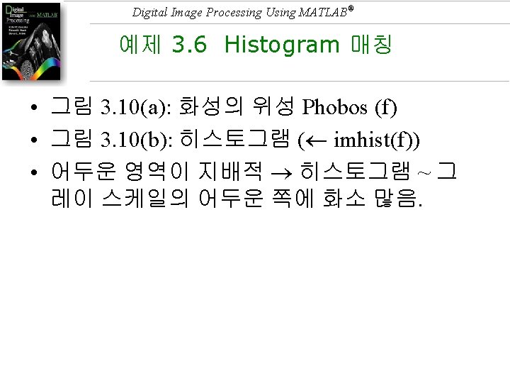
![Digital Image Processing Using MATLAB® >> h = imhist(f) >> ylim([0 25000]) • size(f)](http://slidetodoc.com/presentation_image_h/bd48d3479e1628f8553f19811bcb302a/image-117.jpg "Digital Image Processing Using MATLAB® >> h = imhist(f) >> ylim([0 25000]) • size(f)")
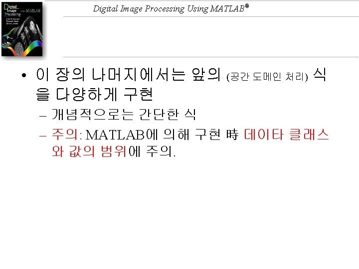
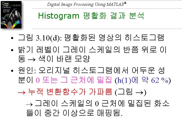
Digital Image Processing Using MATLAB® >> h = imhist(f) >> ylim([0 25000]) • size(f) 1000 683 = 683, 000 pixels • hmax = h(1) 421, 847 pixels 61. 8 % 255 *. 618 = 157
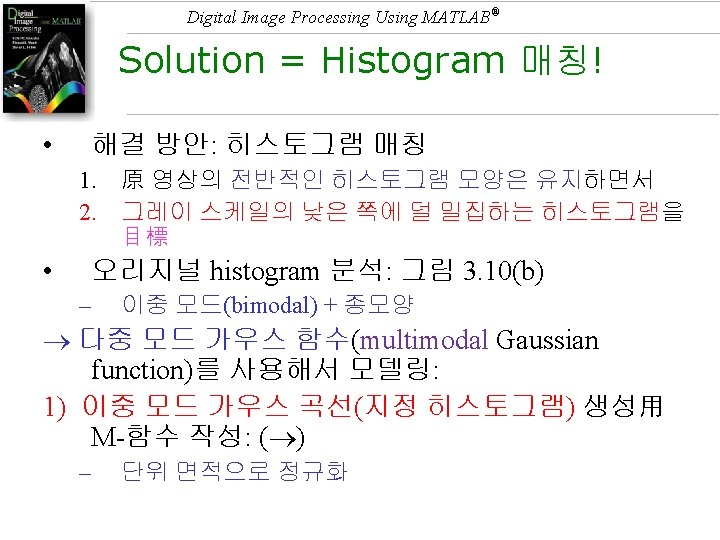

Digital Image Processing Using MATLAB® 지정 히스토그램 생성 M-함수 function p = twomodegauss(m 1, sig 1, m 2, sig 2, A 1, A 2, k) %TWOMODEGAUSS Generates a bimodal Gaussian function. % P = TWOMODEGAUSS(M 1, SIG 1, M 2, SIG 2, A 1, A 2, K) generates a bimodal, % Gaussian-like function in the interval [0, 1]. P is a 256 -element % vector normalized so that SUM(P) equals 1. The mean and standard % deviation of the modes are (M 1, SIG 1) and (M 2, SIG 2), respectively. % A 1 and A 2 are the amplitude values of the two modes. Since the % output is normalized, only the relative values of A 1 and A 2 are % important. K is an offset value that raises the “floor” of the % function. A good set of values to try is M 1 = 0. 15, SIG 1 = 0. 05, % M 2 = 0. 75, SIG 2 = 0. 05, A 1 = 1, A 2 = 0. 07, and K = 0. 002.

Digital Image Processing Using MATLAB® c 1 = A 1 * (1 / ((2 * pi) ^ 0. 5) * sig 1); k 1 = 2 * (sig 1 ^ 2); c 2 = A 2 * (1 / ((2 * pi) ^ 0. 5) * sig 2); k 2 = 2 * (sig 2 ^ 2); z = linspace(0, 1, 256); p = k + c 1 * exp(-((z – m 1). ^ 2). / k 1) +. . . c 2 * exp(-((z – m 2). ^ 2). / k 2); p = p. / sum(p(: ));

Digital Image Processing Using MATLAB® >> p = twomodegauss(0. 15, 0. 05, 0. 75, 0. 05, 1, 0. 07, 0. 002); – function p = twomodegauss(m 1, sig 1, m 2, sig 2, A 1, A 2, k) >> figure, plot(p)
 Histogram 그리는 M-함수 작성 • 대화형: 입력 from")
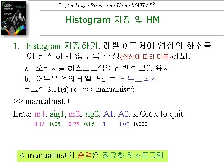
Digital Image Processing Using MATLAB® 2) Histogram 그리는 M-함수 작성 • 대화형: 입력 from 키보드 • 함수 이름: manualhist • 함수 기능: i) twomodegauss(…)를 호출해서 가우스 함수를 생성하고, ii) 그린다. • 함수 input과 str 2 num의 설명: § 2. 10. 5 >> user_entry = input('prompt', 's') – returns the entered string as a text variable rather than as a variable name or numerical value. – 쉼표 또는 공백에 의해 요소를 분리시킬 수 있는 문자 열을 받아들임.

Digital Image Processing Using MATLAB® function p = manualhist %MANUALHIST Generates a two-mode histogram interactively. % P = MANUALHIST generates a two-mode histogram using % TWOMODEGAUSS(m 1, sig 1, m 2, sig 2, A 1, A 2, k). m 1 and m 2 are the % means of the two modes and must be in the range [0, 1]. sig 1 and % sig 2 are the standard deviations of the two modes. A 1 and A 2 are % amplitude values, and k is an offset value that raised the % "floor" of histogram. The number of elements in the histogram % vector P is 256 and sum(P) is normalized to 1. MANUALHIST % repeatedly prompts for the parameters and plots the resulting % histogram until the user types an 'x' to quit, and then it returns % the last histogram computed.

Digital Image Processing Using MATLAB® % Initialize. repeats = true; quitnow = ‘x’; % Compute a default histogram in case the user quits before % estimating at least one histogram. p = twomodegauss(0. 15, 0. 05, 0. 75, 0. 05, 1, 0. 07, 0. 002); % Cycle until an x is input.

Digital Image Processing Using MATLAB® while repeats s = input('Enter m 1, sig 1, m 2, sig 2, A 1, A 2, k, OR x to quit: n', 's'); if s == quitnow break end v = str 2 num(s); if numel(v) ~= 7 disp(‘Incorrect number of inputs. n’) continue end p = twomodegauss(v(1), v(2), v(3), v(4), v(5), v(6), v(7)); figure, plot(p) xlim([0 255]) end
; % ans")
Digital Image Processing Using MATLAB® 2. HM: >> g = histeq(f, ans); % ans = norm. histogram >> imshow(g), imhist(g) % Figs. 3. 11 (b), (c)
 transforms the intensity image")
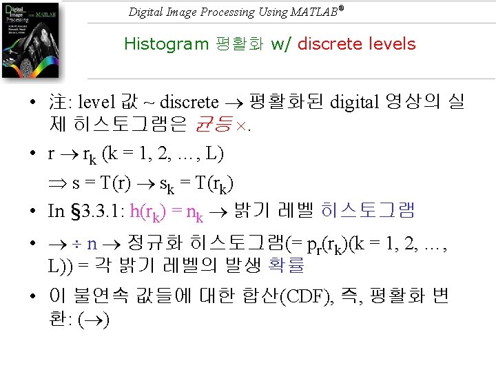
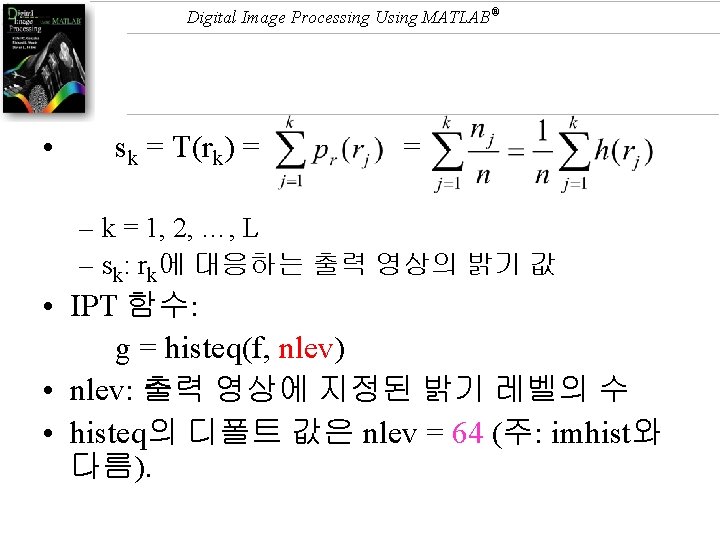
Digital Image Processing Using MATLAB® histeq J = histeq(I, hgram) transforms the intensity image I so that the histogram of the output intensity image J with length(hgram) bins approximately matches hgram. The vector hgram should contain integer counts for equally spaced bins with intensity values in the appropriate range: [0, 1] for images of class double, [0, 255] for images of class uint 8, and [0, 65535] for images of class uint 16. histeq automatically scales hgram so that sum(hgram) = prod(size(I)). The histogram of J will better match hgram when length(hgram) is much smaller than the number of discrete levels in I. J = histeq(I, n) transforms the intensity image I, returning in J an intensity image with n discrete gray levels. A roughly equal number of pixels is mapped to each of the n levels in J, so that the histogram of J is approximately flat. (The histogram of J is flatter when n is much smaller than the number of discrete levels in I. ) The default value for n is 64.

Digital Image Processing Using MATLAB®

Digital Image Processing Using MATLAB® Lena 영상에 대한 실험 original desired

Digital Image Processing Using MATLAB® >> manualhist Enter m 1, sig 1, m 2, sig 2, A 1, A 2, k, OR x to quit: 0. 15 0. 05 0. 75 0. 05 1 0. 07 0. 002 Enter m 1, sig 1, m 2, sig 2, A 1, A 2, k, OR x to quit: x >> g = histeq(f 1, ans); >> imshow(g), imhist(g)

Digital Image Processing Using MATLAB® What is the problem? more than 3 modes!

Digital Image Processing Using MATLAB®
 • threemodegauss(m 1, s 1, m 2, s")
Digital Image Processing Using MATLAB® (cont’d) • threemodegauss(m 1, s 1, m 2, s 2, m 3, s 3, A 1, A 2, A 3 , k), fourmodegauss(…) 等을 작성 할 것 -- 필 수 • You may need to write a function manualhist 3 Gauss(…) which will call the function threemodegauss(…), manualhist 4 Gauss(…) which will call the function fourmodegauss(…), and so on. • 실험결과에 대한 분석 중요.

Digital Image Processing Using MATLAB® Batch file 작성해서 Cell mode로 실험! f 2: 원하는 히스토그램을 갖는 영상

Digital Image Processing Using MATLAB®
- Slides: 137