DIGITAL IMAGE PROCESSING Lecture 9 Features detection and

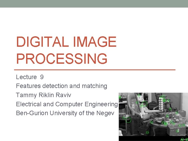
DIGITAL IMAGE PROCESSING Lecture 9 Features detection and matching Tammy Riklin Raviv Electrical and Computer Engineering Ben-Gurion University of the Negev

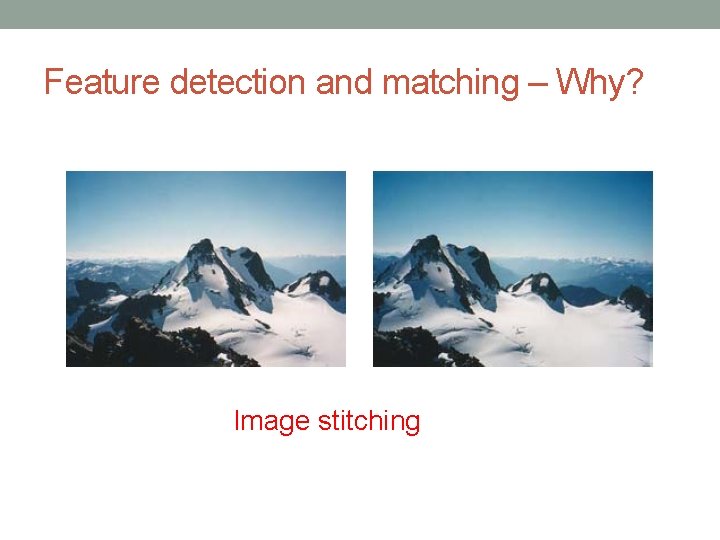
Feature detection and matching – Why? Image stitching

3 Image Stitching [ Brown, Szeliski, Winder CVPR 2005 ]

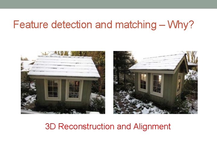
Feature detection and matching – Why? 3 D Reconstruction and Alignment

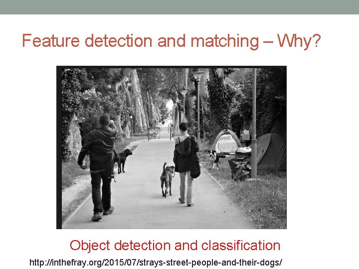
Feature detection and matching – Why? Object detection and classification http: //inthefray. org/2015/07/strays-street-people-and-their-dogs/

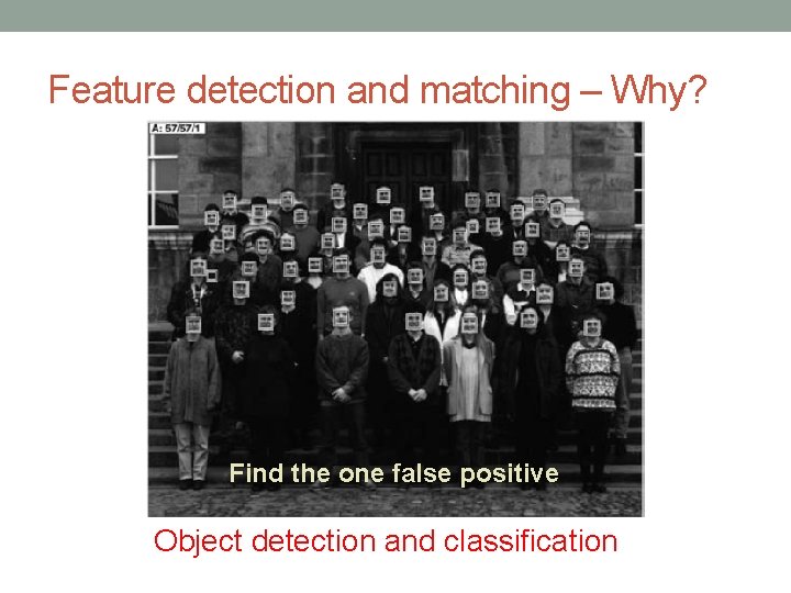
Feature detection and matching – Why? Find the one false positive Object detection and classification

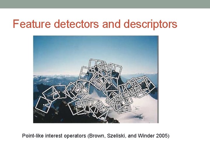
Feature detectors and descriptors Point-like interest operators (Brown, Szeliski, and Winder 2005)

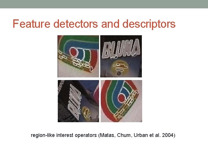
Feature detectors and descriptors region-like interest operators (Matas, Chum, Urban et al. 2004)

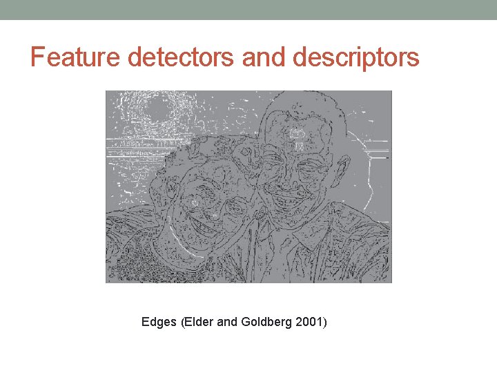
Feature detectors and descriptors Edges (Elder and Goldberg 2001)

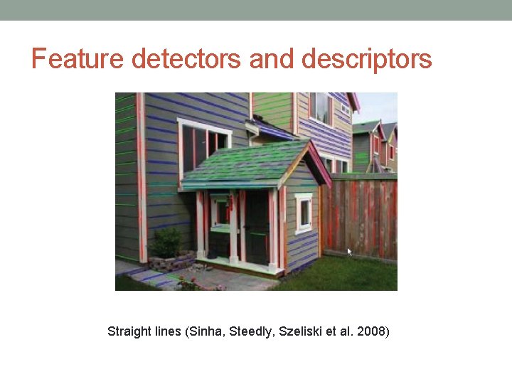
Feature detectors and descriptors Straight lines (Sinha, Steedly, Szeliski et al. 2008)

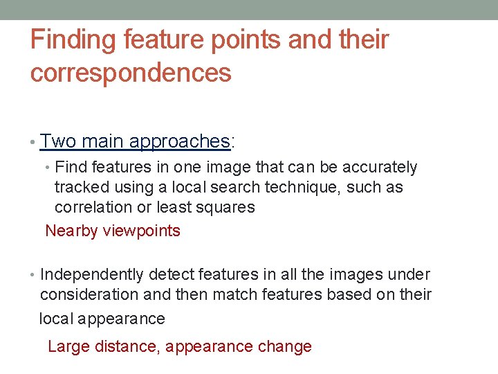
Finding feature points and their correspondences • Two main approaches: • Find features in one image that can be accurately tracked using a local search technique, such as correlation or least squares Nearby viewpoints • Independently detect features in all the images under consideration and then match features based on their local appearance Large distance, appearance change

Feature detection and matching • Feature detection (extraction) • Feature description • Feature matching • Feature tracking

Feature detection and matching • Feature detection (extraction) • each image is searched for locations that are likely to match well in other images. • Feature description • Feature matching • Feature tracking

Feature detection and matching • Feature detection (extraction) • Feature description • each region around detected keypoint locations is converted into a more compact and stable (invariant) descriptor that can be matched against other descriptors. • Feature matching • Feature tracking

Feature detection and matching • Feature detection (extraction) • Feature description • Feature matching • efficiently searches for likely matching candidates in other images. • Feature tracking

Feature detection and matching • Feature detection (extraction) • Feature description • Feature matching • Feature tracking • alternative to the third stage that only searches a small neighborhood around each detected feature and is therefore more suitable for video processing.

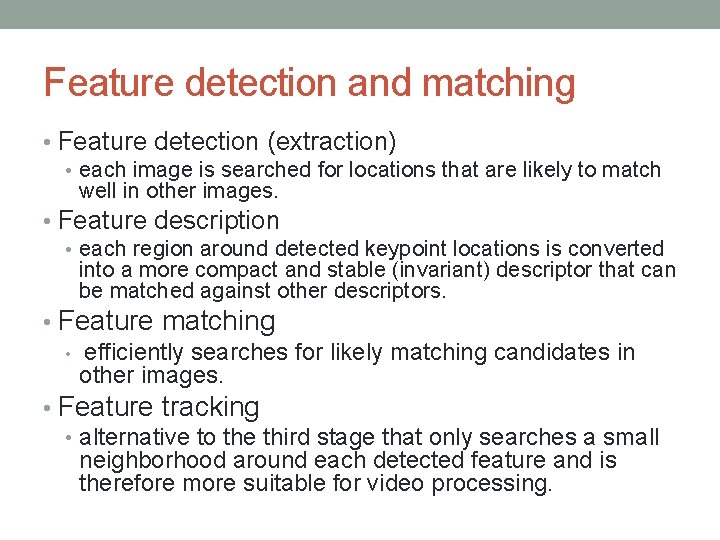
Feature detection and matching • Feature detection (extraction) • each image is searched for locations that are likely to match well in other images. • Feature description • each region around detected keypoint locations is converted into a more compact and stable (invariant) descriptor that can be matched against other descriptors. • Feature matching • efficiently searches for likely matching candidates in other images. • Feature tracking • alternative to the third stage that only searches a small neighborhood around each detected feature and is therefore more suitable for video processing.

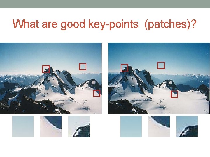
What are good key-points (patches)?

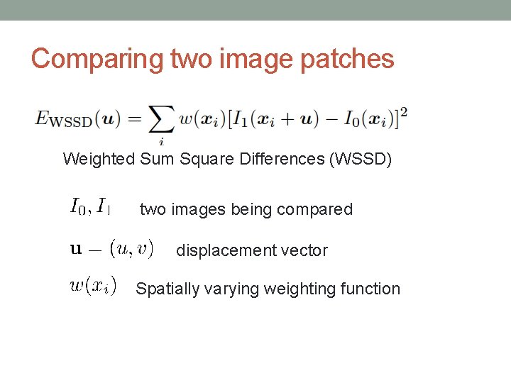
Comparing two image patches Weighted Sum Square Differences (WSSD) two images being compared displacement vector Spatially varying weighting function

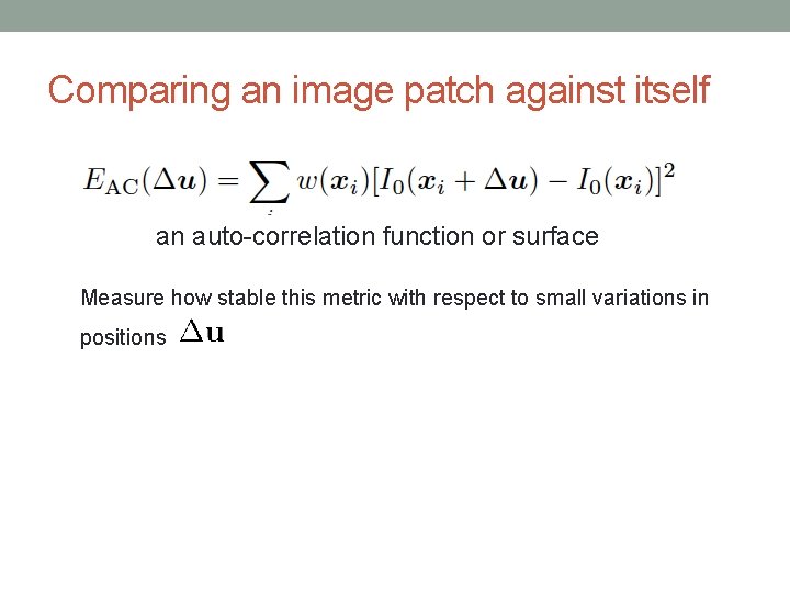
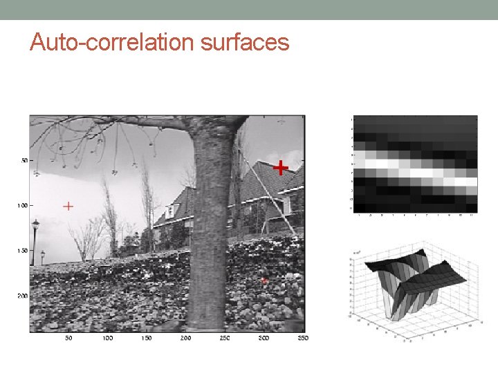
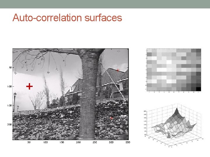
Comparing an image patch against itself an auto-correlation function or surface Measure how stable this metric with respect to small variations in positions

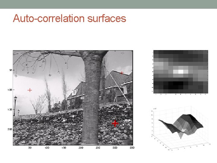
Auto-correlation surfaces +

Auto-correlation surfaces +

Auto-correlation surfaces +

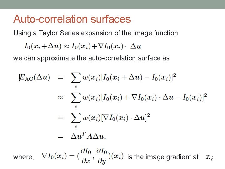
Auto-correlation surfaces Using a Taylor Series expansion of the image function we can approximate the auto-correlation surface as where, is the image gradient at .

Auto-correlation surfaces Calculating the gradient: Classic Harris detector: [-2 -1 0 1 2] filter. Modern variants: convolve the image with horizontal and vertical derivatives of a Gaussian (typically with ).

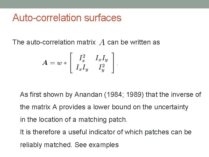
Auto-correlation surfaces The auto-correlation matrix can be written as As first shown by Anandan (1984; 1989) that the inverse of the matrix A provides a lower bound on the uncertainty in the location of a matching patch. It is therefore a useful indicator of which patches can be reliably matched. See examples

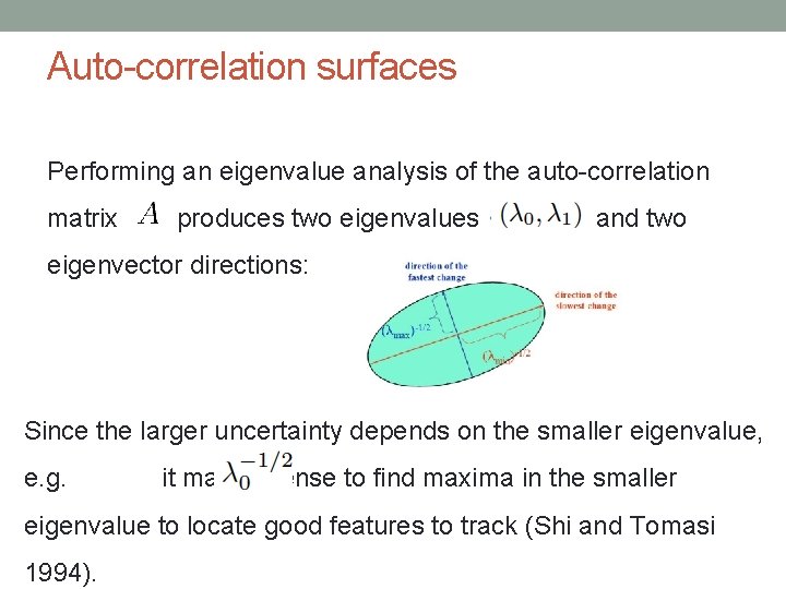
Auto-correlation surfaces Performing an eigenvalue analysis of the auto-correlation matrix produces two eigenvalues and two eigenvector directions: Since the larger uncertainty depends on the smaller eigenvalue, e. g. it makes sense to find maxima in the smaller eigenvalue to locate good features to track (Shi and Tomasi 1994).

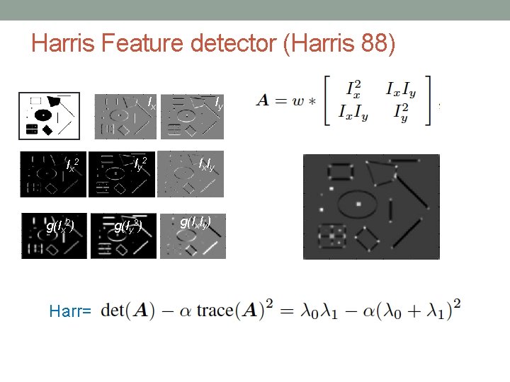
Harris Feature detector (Harris 88) Ix Ix 2 g(Ix 2) Harr= Iy 2 g(Iy 2) Iy Ix Iy g(Ix. Iy)

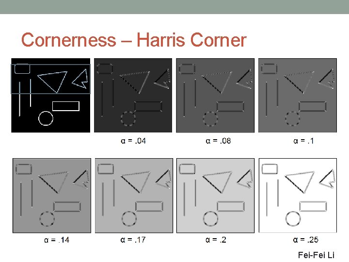
Cornerness – Harris Corner Fei-Fei Li

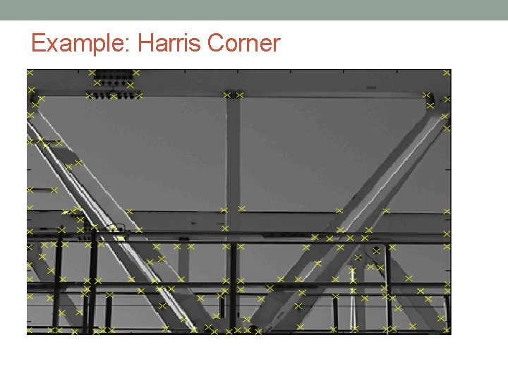
Example: Harris Corner

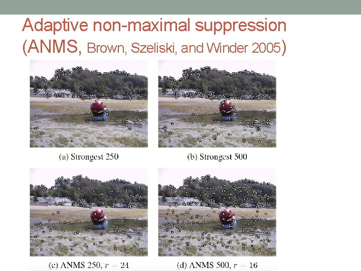
Adaptive non-maximal suppression (ANMS, Brown, Szeliski, and Winder 2005)

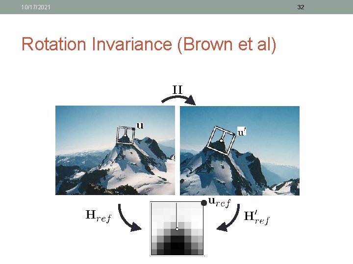
10/17/2021 Rotation Invariance (Brown et al) 32

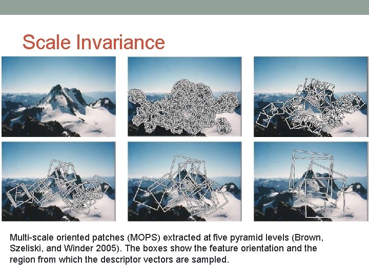
Scale Invariance Multi-scale oriented patches (MOPS) extracted at five pyramid levels (Brown, Szeliski, and Winder 2005). The boxes show the feature orientation and the region from which the descriptor vectors are sampled.

10/17/2021 34 Ideas from Brown’s Multi-Scale Oriented Patches • 1. Detect an interesting patch with an interest operator. Patches are translation invariant. • 2. Determine its dominant orientation. • 3. Rotate the patch so that the dominant orientation points upward. This makes the patches rotation invariant. • 4. Do this at multiple scales, converting them all to one scale through sampling. • 5. Convert to illumination “invariant” form

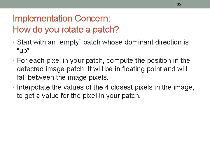
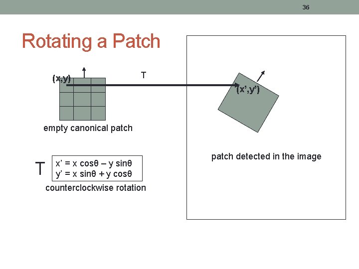
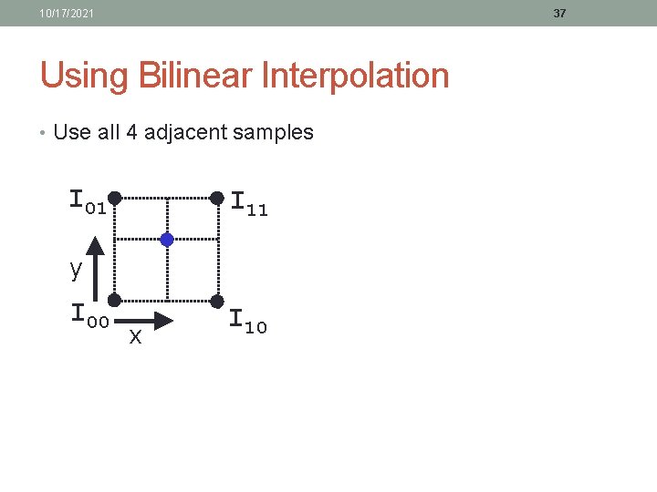
35 Implementation Concern: How do you rotate a patch? • Start with an “empty” patch whose dominant direction is “up”. • For each pixel in your patch, compute the position in the detected image patch. It will be in floating point and will fall between the image pixels. • Interpolate the values of the 4 closest pixels in the image, to get a value for the pixel in your patch.

36 Rotating a Patch (x, y) T (x’, y’) empty canonical patch T x’ = x cosθ – y sinθ y’ = x sinθ + y cosθ counterclockwise rotation patch detected in the image

10/17/2021 37 Using Bilinear Interpolation • Use all 4 adjacent samples I 01 I 11 y I 00 x I 10

10/17/2021 38 SIFT: Motivation • The Harris operator is not invariant to scale and correlation is not invariant to rotation 1. • For better image matching, Lowe’s goal was to develop an interest operator that is invariant to scale and rotation. • Also, Lowe aimed to create a descriptor that was robust to the variations corresponding to typical viewing conditions. The descriptor is the most-used part of SIFT. 1 But Schmid and Mohr developed a rotation invariant descriptor for it in 1997.

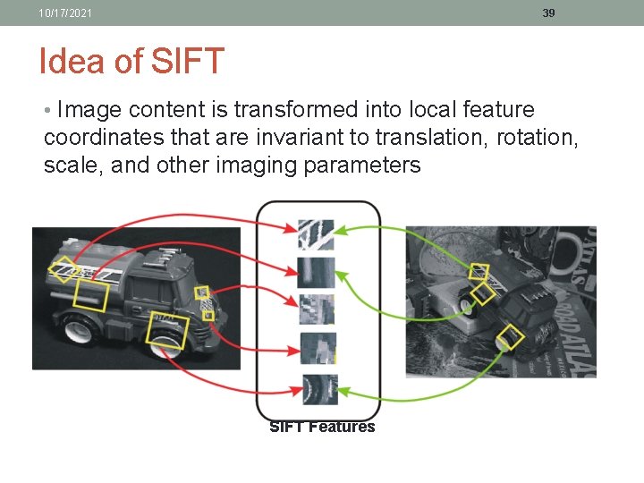
10/17/2021 39 Idea of SIFT • Image content is transformed into local feature coordinates that are invariant to translation, rotation, scale, and other imaging parameters SIFT Features

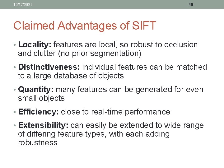
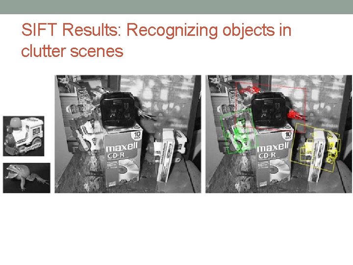
10/17/2021 40 Claimed Advantages of SIFT • Locality: features are local, so robust to occlusion and clutter (no prior segmentation) • Distinctiveness: individual features can be matched to a large database of objects • Quantity: many features can be generated for even small objects • Efficiency: close to real-time performance • Extensibility: can easily be extended to wide range of differing feature types, with each adding robustness

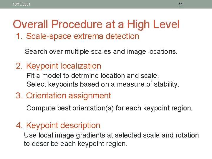
10/17/2021 41 Overall Procedure at a High Level 1. Scale-space extrema detection Search over multiple scales and image locations. 2. Keypoint localization Fit a model to detrmine location and scale. Select keypoints based on a measure of stability. 3. Orientation assignment Compute best orientation(s) for each keypoint region. 4. Keypoint description Use local image gradients at selected scale and rotation to describe each keypoint region.

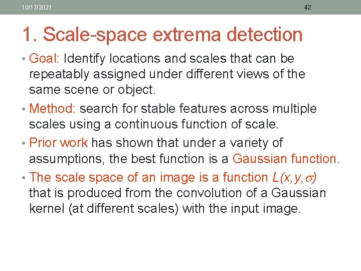
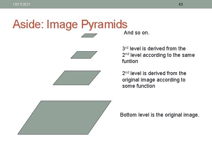
10/17/2021 42 1. Scale-space extrema detection • Goal: Identify locations and scales that can be repeatably assigned under different views of the same scene or object. • Method: search for stable features across multiple scales using a continuous function of scale. • Prior work has shown that under a variety of assumptions, the best function is a Gaussian function. • The scale space of an image is a function L(x, y, ) that is produced from the convolution of a Gaussian kernel (at different scales) with the input image.

10/17/2021 43 Aside: Image Pyramids And so on. 3 rd level is derived from the 2 nd level according to the same funtion 2 nd level is derived from the original image according to some function Bottom level is the original image.

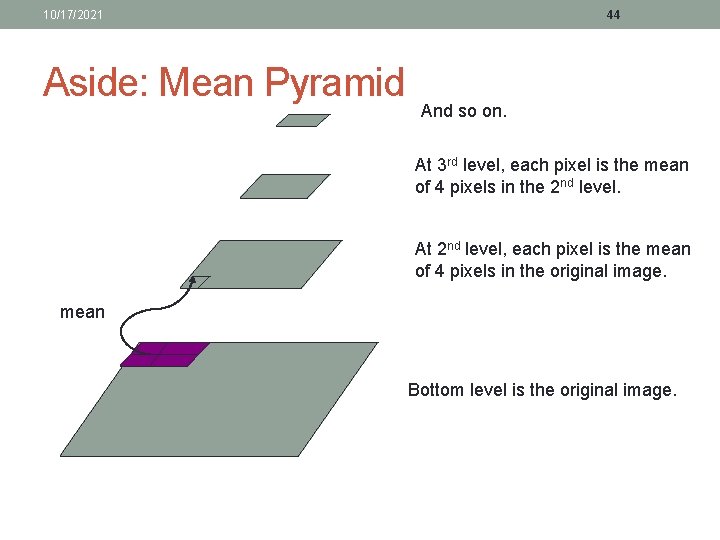
10/17/2021 Aside: Mean Pyramid 44 And so on. At 3 rd level, each pixel is the mean of 4 pixels in the 2 nd level. At 2 nd level, each pixel is the mean of 4 pixels in the original image. mean Bottom level is the original image.

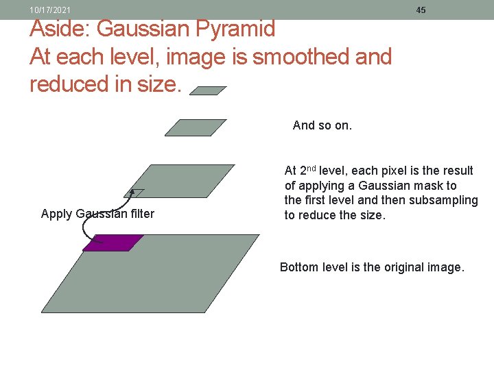
10/17/2021 45 Aside: Gaussian Pyramid At each level, image is smoothed and reduced in size. And so on. Apply Gaussian filter At 2 nd level, each pixel is the result of applying a Gaussian mask to the first level and then subsampling to reduce the size. Bottom level is the original image.

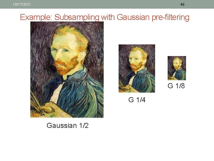
10/17/2021 46 Example: Subsampling with Gaussian pre-filtering G 1/8 G 1/4 Gaussian 1/2

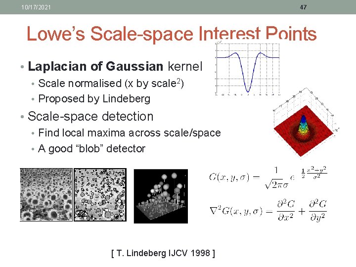
10/17/2021 47 Lowe’s Scale-space Interest Points • Laplacian of Gaussian kernel • Scale normalised (x by scale 2) • Proposed by Lindeberg • Scale-space detection • Find local maxima across scale/space • A good “blob” detector [ T. Lindeberg IJCV 1998 ]

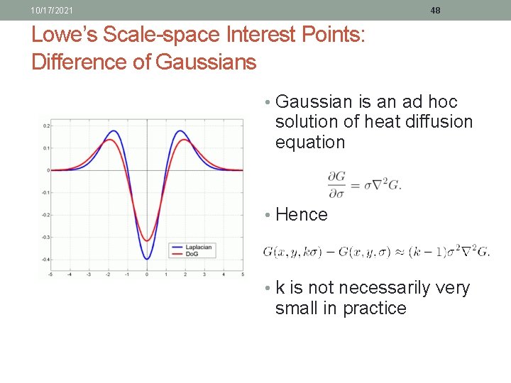
10/17/2021 48 Lowe’s Scale-space Interest Points: Difference of Gaussians • Gaussian is an ad hoc solution of heat diffusion equation • Hence • k is not necessarily very small in practice

10/17/2021 49 Lowe’s Pyramid Scheme • Scale space is separated into octaves: • Octave 1 uses scale • Octave 2 uses scale 2 • etc. • In each octave, the initial image is repeatedly convolved with Gaussians to produce a set of scale space images. • Adjacent Gaussians are subtracted to produce the DOG • After each octave, the Gaussian image is down-sampled by a factor of 2 to produce an image ¼ the size to start the next level.

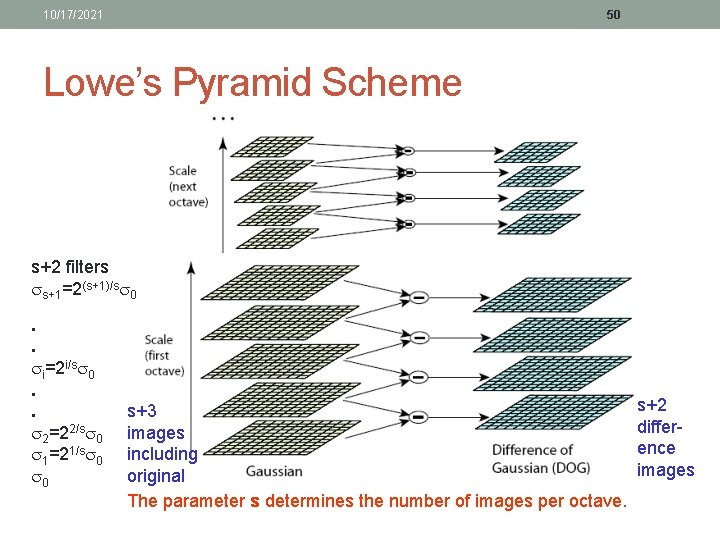
10/17/2021 50 Lowe’s Pyramid Scheme s+2 filters s+1=2(s+1)/s 0. . i=2 i/s 0. . 2=22/s 0 1=21/s 0 0 s+3 images including original The parameter s determines the number of images per octave. s+2 difference images

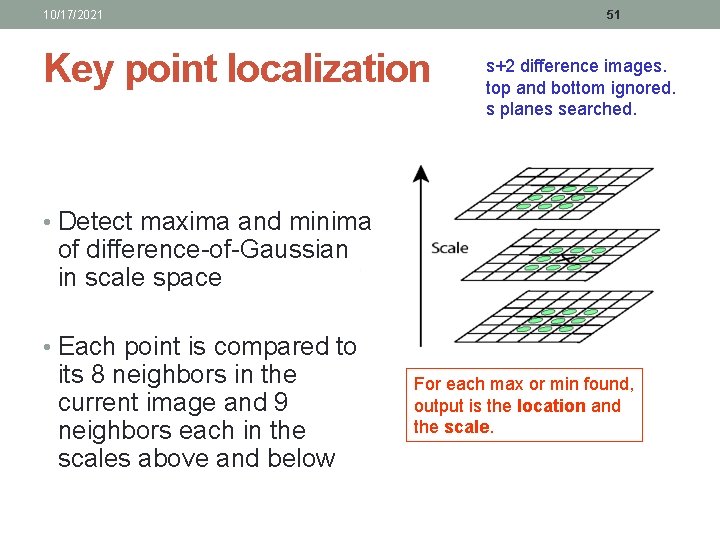
10/17/2021 51 Key point localization s+2 difference images. top and bottom ignored. s planes searched. • Detect maxima and minima of difference-of-Gaussian in scale space • Each point is compared to its 8 neighbors in the current image and 9 neighbors each in the scales above and below For each max or min found, output is the location and the scale.

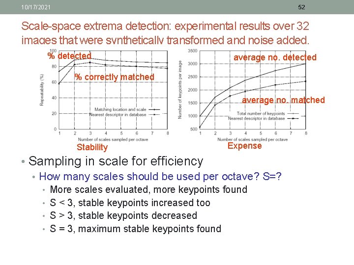
10/17/2021 52 Scale-space extrema detection: experimental results over 32 images that were synthetically transformed and noise added. % detected average no. detected % correctly matched average no. matched Stability Expense • Sampling in scale for efficiency • How many scales should be used per octave? S=? • • More scales evaluated, more keypoints found S < 3, stable keypoints increased too S > 3, stable keypoints decreased S = 3, maximum stable keypoints found

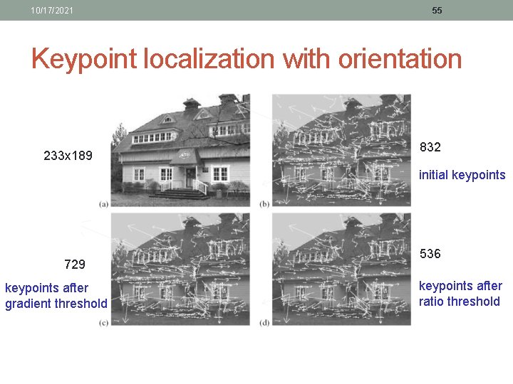
10/17/2021 53 2. Keypoint localization • Once a keypoint candidate is found, perform a detailed fit to nearby data to determine • location, scale, and ratio of principal curvatures • In initial work keypoints were found at location and scale of a central sample point. • In newer work, they fit a 3 D quadratic function to improve interpolation accuracy. • The Hessian matrix was used to eliminate edge responses.

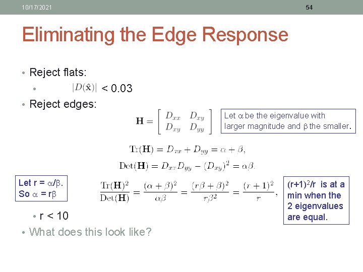
10/17/2021 54 Eliminating the Edge Response • Reject flats: • < 0. 03 • Reject edges: Let be the eigenvalue with larger magnitude and the smaller. Let r = /. So = r • r < 10 • What does this look like? (r+1)2/r is at a min when the 2 eigenvalues are equal.

10/17/2021 55 Keypoint localization with orientation 233 x 189 832 initial keypoints 729 keypoints after gradient threshold 536 keypoints after ratio threshold

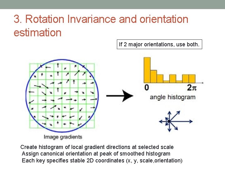
3. Rotation Invariance and orientation estimation If 2 major orientations, use both. Create histogram of local gradient directions at selected scale Assign canonical orientation at peak of smoothed histogram Each key specifies stable 2 D coordinates (x, y, scale, orientation)

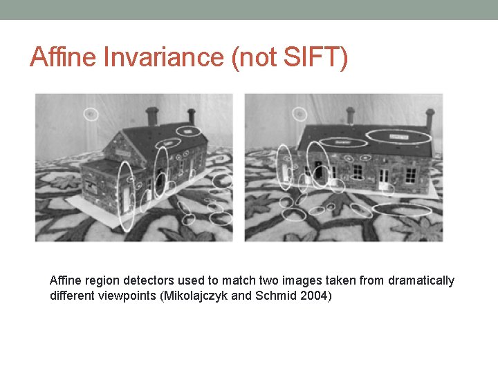
Affine Invariance (not SIFT) Affine region detectors used to match two images taken from dramatically different viewpoints (Mikolajczyk and Schmid 2004)

10/17/2021 58 4. Keypoint Descriptors • At this point, each keypoint has • location • scale • orientation • Next is to compute a descriptor for the local image region about each keypoint that is • highly distinctive • invariant as possible to variations such as changes in viewpoint and illumination

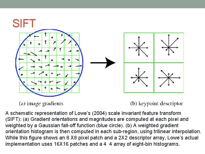
SIFT A schematic representation of Lowe’s (2004) scale invariant feature transform (SIFT): (a) Gradient orientations and magnitudes are computed at each pixel and weighted by a Gaussian fall-off function (blue circle). (b) A weighted gradient orientation histogram is then computed in each sub-region, using trilinear interpolation. While this figure shows an 8 X 8 pixel patch and a 2 X 2 descriptor array, Lowe’s actual implementation uses 16 X 16 patches and a 4 4 array of eight-bin histograms.

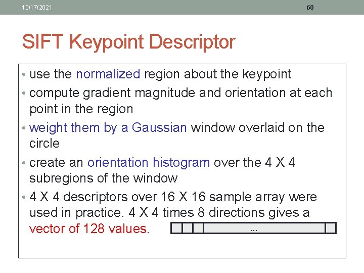
10/17/2021 60 SIFT Keypoint Descriptor • use the normalized region about the keypoint • compute gradient magnitude and orientation at each point in the region • weight them by a Gaussian window overlaid on the circle • create an orientation histogram over the 4 X 4 subregions of the window • 4 X 4 descriptors over 16 X 16 sample array were used in practice. 4 X 4 times 8 directions gives a. . . vector of 128 values.

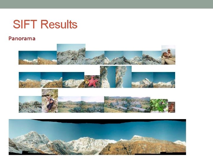
SIFT Results

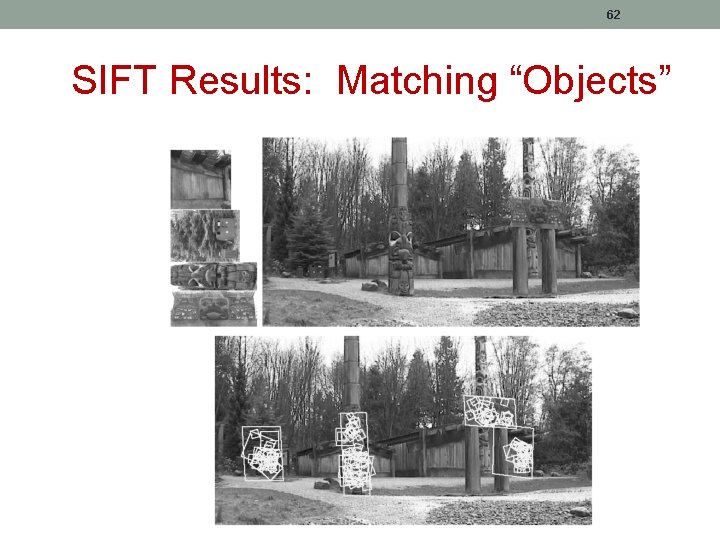
62 SIFT Results: Matching “Objects”

SIFT Results: Recognizing objects in clutter scenes

Feature Descriptors (other than SIFT) • Multiscale Oriented Patches (MOPs). • Scale invariant feature transform (MSERs) • PCA-SIFT • Gradient location-orientation histogram (GLOH). • Histograms of Oriented Gradients (HOGs) • Speeded Up Robust Features (SURF) • and many others … • (e. g. BRISK )

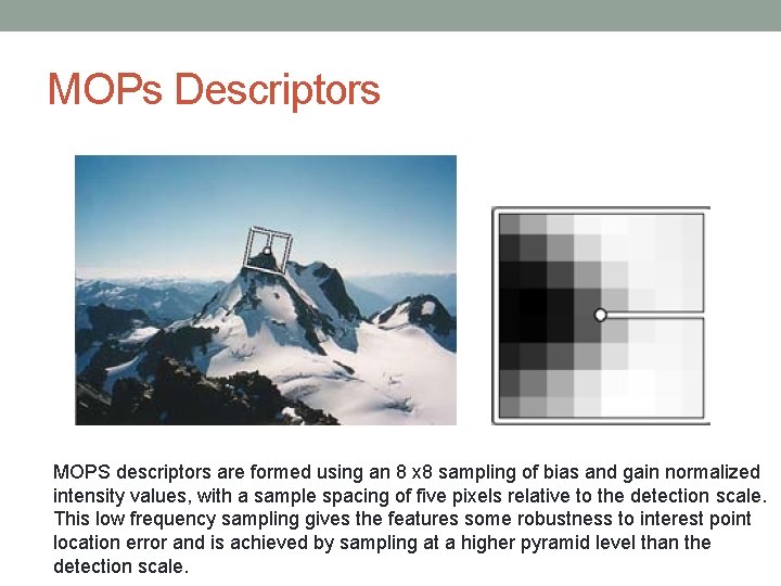
MOPs Descriptors MOPS descriptors are formed using an 8 x 8 sampling of bias and gain normalized intensity values, with a sample spacing of five pixels relative to the detection scale. This low frequency sampling gives the features some robustness to interest point location error and is achieved by sampling at a higher pyramid level than the detection scale.

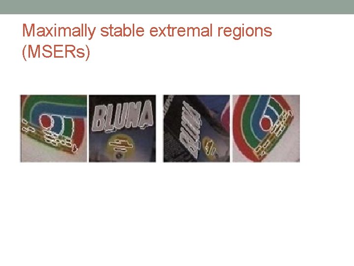
Maximally stable extremal regions (MSERs)

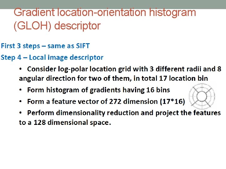
Gradient location-orientation histogram (GLOH) descriptor

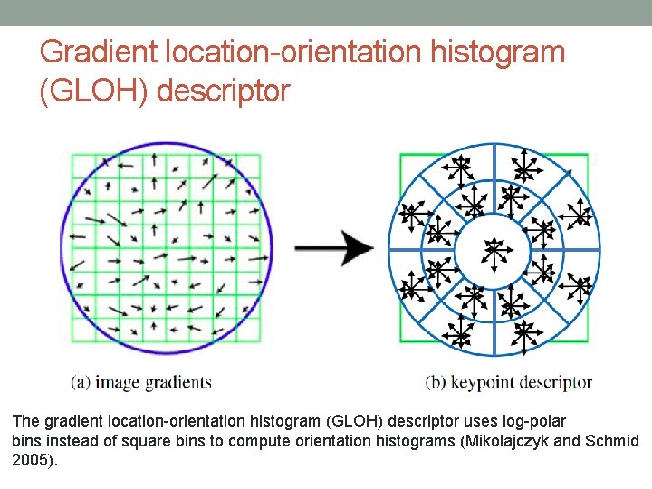
Gradient location-orientation histogram (GLOH) descriptor The gradient location-orientation histogram (GLOH) descriptor uses log-polar bins instead of square bins to compute orientation histograms (Mikolajczyk and Schmid 2005).

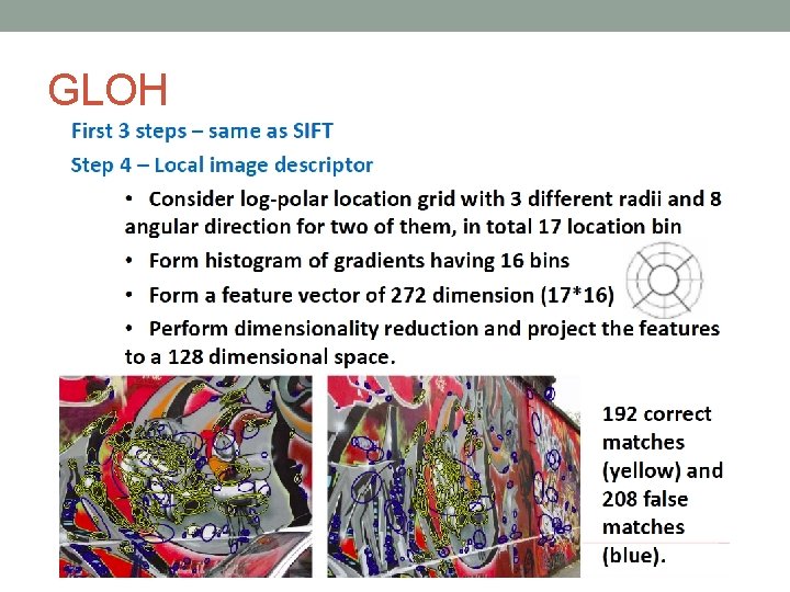
GLOH

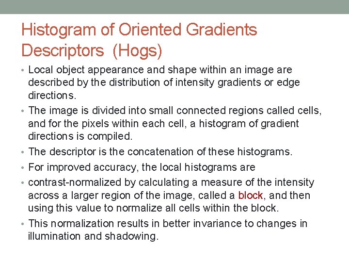
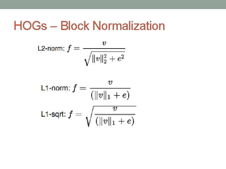
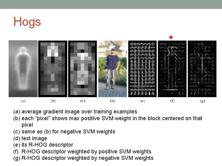
Histogram of Oriented Gradients Descriptors (Hogs) • Local object appearance and shape within an image are • • • described by the distribution of intensity gradients or edge directions. The image is divided into small connected regions called cells, and for the pixels within each cell, a histogram of gradient directions is compiled. The descriptor is the concatenation of these histograms. For improved accuracy, the local histograms are contrast-normalized by calculating a measure of the intensity across a larger region of the image, called a block, and then using this value to normalize all cells within the block. This normalization results in better invariance to changes in illumination and shadowing.

HOGs – Block Normalization

Hogs * (a) average gradient image over training examples (b) each “pixel” shows max positive SVM weight in the block centered on that pixel (c) same as (b) for negative SVM weights (d) test image (e) its R-HOG descriptor (f) R-HOG descriptor weighted by positive SVM weights (g) R-HOG descriptor weighted by negative SVM weights

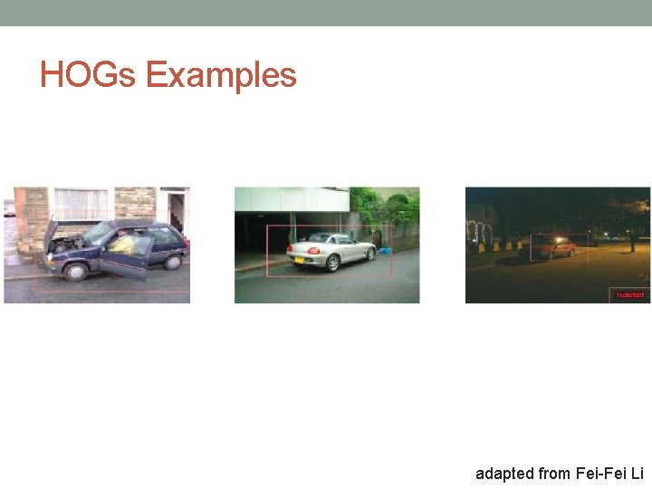
HOGs Examples adapted from Fei-Fei Li

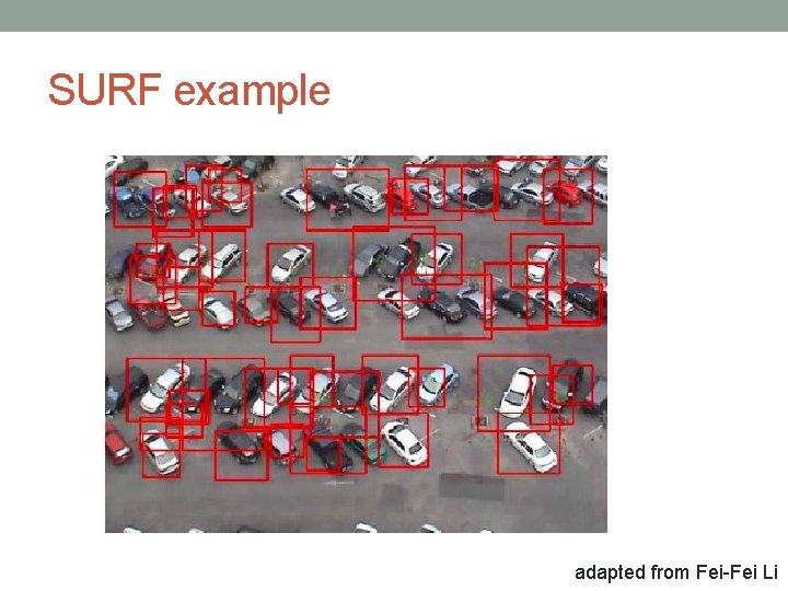
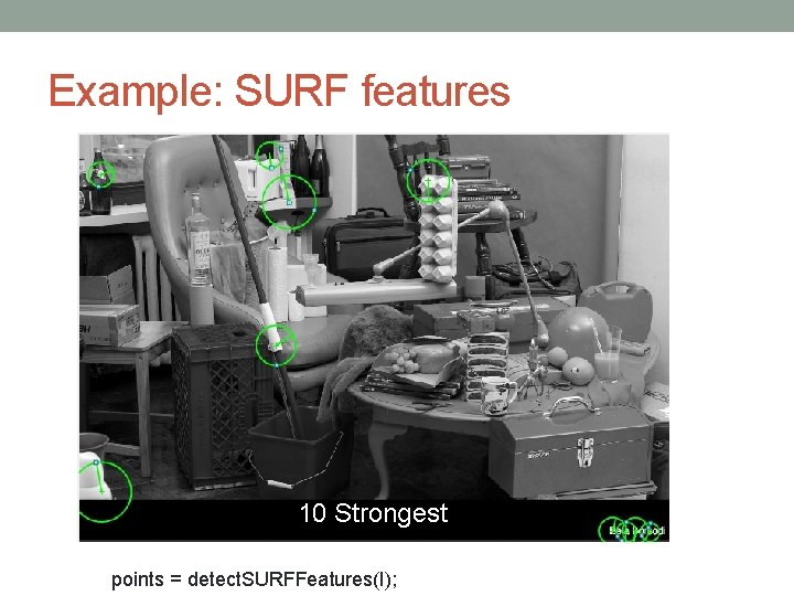
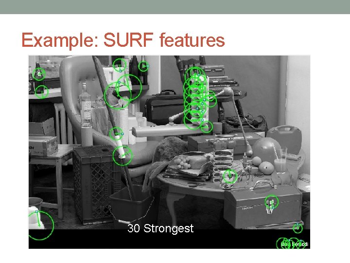
SURF example adapted from Fei-Fei Li

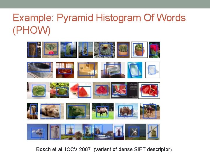
Example: Pyramid Histogram Of Words (PHOW) Bosch et al, ICCV 2007 (variant of dense SIFT descriptor)

Features in Matlab [FEATURES, VALID_POINTS] = extract. Features(I, POINTS, Name, Value)

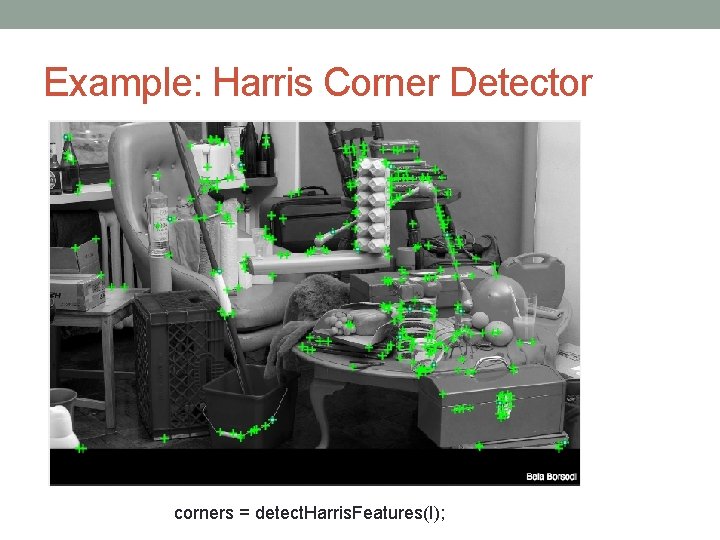
Example: Harris Corner Detector corners = detect. Harris. Features(I);

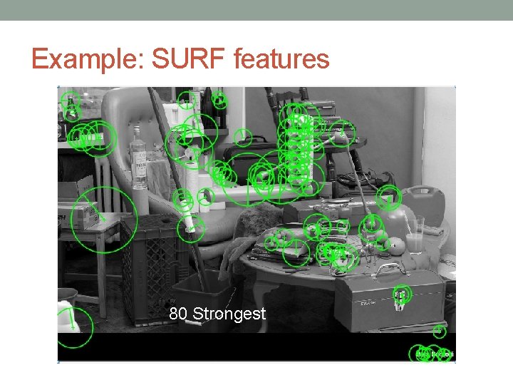
Example: SURF features 10 Strongest points = detect. SURFFeatures(I);

Example: SURF features 30 Strongest

Example: SURF features 80 Strongest

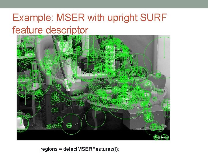
Example: MSER with upright SURF feature descriptor regions = detect. MSERFeatures(I);

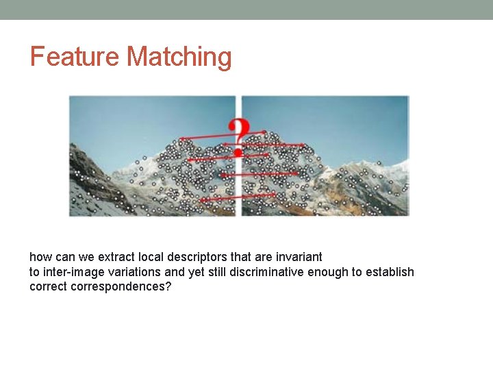
Feature Matching how can we extract local descriptors that are invariant to inter-image variations and yet still discriminative enough to establish correct correspondences?

Matching strategy and error rates • Context and application dependent • matching a pair of images with large overlap • object detection • Euclidean distances in feature space can be directly used for ranking potential matches. • Thresholding

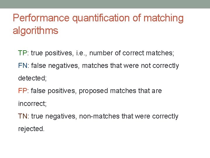
Performance quantification of matching algorithms TP: true positives, i. e. , number of correct matches; FN: false negatives, matches that were not correctly detected; FP: false positives, proposed matches that are incorrect; TN: true negatives, non-matches that were correctly rejected.

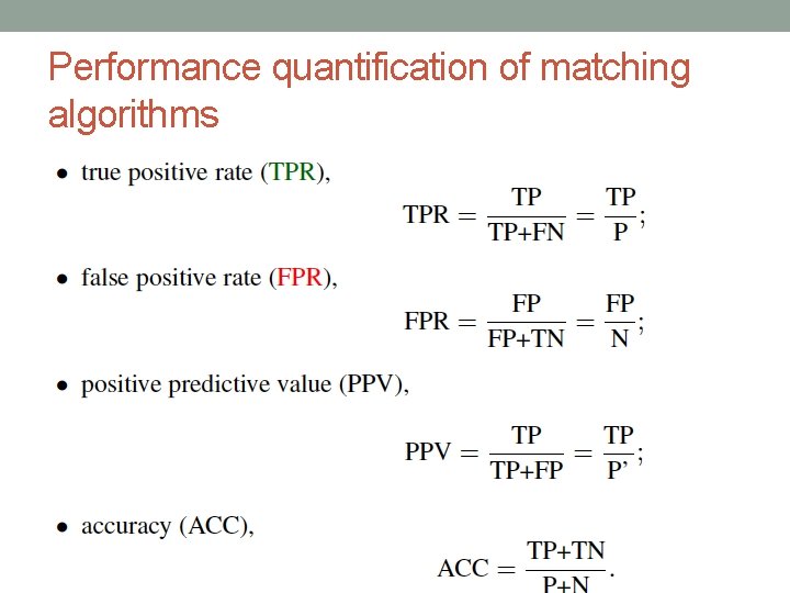
Performance quantification of matching algorithms

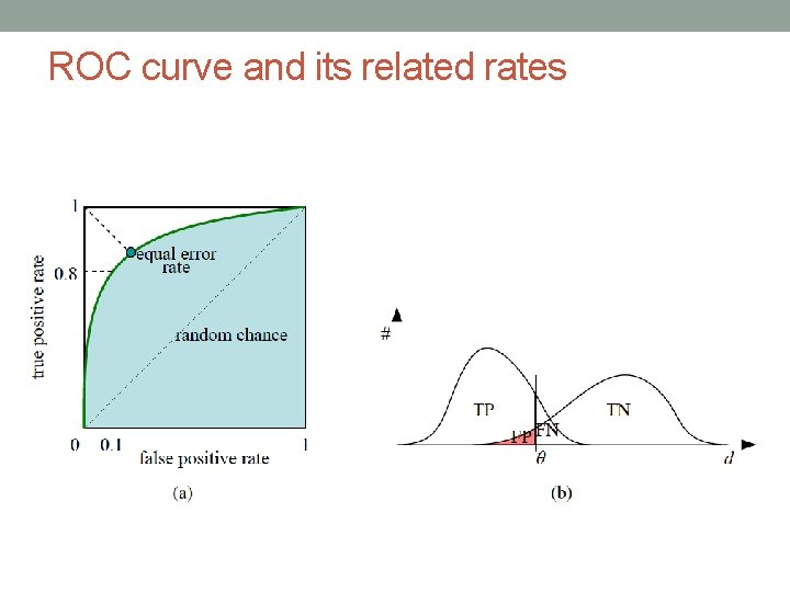
ROC curve and its related rates

Efficient Matching • Multi-dimensional search tree • Hash table

Next Classes • 3 D reconstruction • Image Segmentation • Object detection (+some Machine Learning) • Intro to Deep Learning