Digital Image Processing Lecture 4 Image Enhancement Point

Digital Image Processing Lecture 4: Image Enhancement: Point. Prof. Processing Charlene Tsai

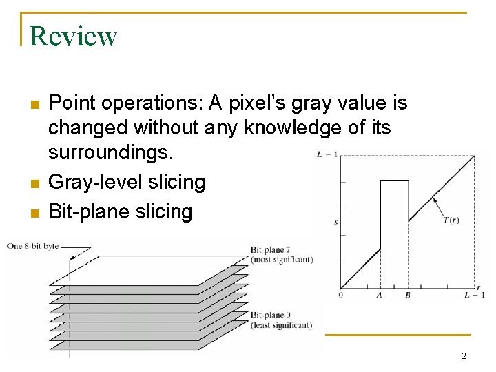
Review n n n Point operations: A pixel’s gray value is changed without any knowledge of its surroundings. Gray-level slicing Bit-plane slicing 2

Arithmetic Operations n n May perform arithmetic operations (+, , *, /, neg) on an image. Always make sure the new value, as well as the intermediate value, is within the intensity range. Operations are straightforward. Matlab commands: imadd, imsubtract, etc. . 3

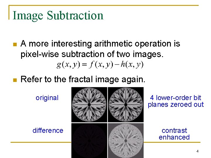
Image Subtraction n A more interesting arithmetic operation is pixel-wise subtraction of two images. n Refer to the fractal image again. original 4 lower-order bit planes zeroed out difference contrast enhanced 4

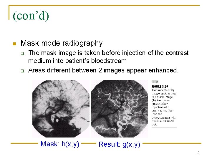
(con’d) n Mask mode radiography q q The mask image is taken before injection of the contrast medium into patient’s bloodstream Areas different between 2 images appear enhanced. Mask: h(x, y) Result: g(x, y) 5

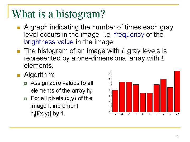
What is a histogram? n n n A graph indicating the number of times each gray level occurs in the image, i. e. frequency of the brightness value in the image The histogram of an image with L gray levels is represented by a one-dimensional array with L elements. Algorithm: q q Assign zero values to all elements of the array hf; For all pixels (x, y) of the image f, increment hf[f(x, y)] by 1. 6

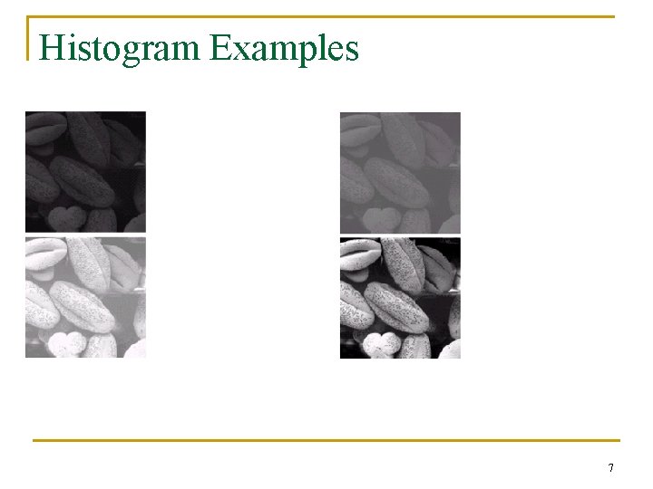
Histogram Examples 7

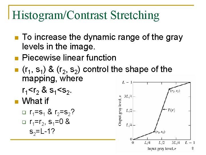
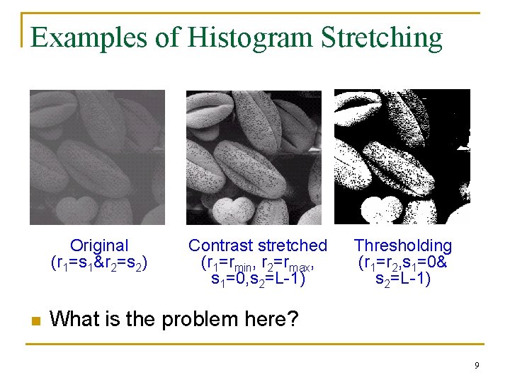
Histogram/Contrast Stretching n n To increase the dynamic range of the gray levels in the image. Piecewise linear function (r 1, s 1) & (r 2, s 2) control the shape of the mapping, where r 1<r 2 & s 1<s 2. What if q q r 1=s 1 & r 2=s 2? r 1=r 2, s 1=0 & s 2=L-1? 8

Examples of Histogram Stretching Original (r 1=s 1&r 2=s 2) n Contrast stretched (r 1=rmin, r 2=rmax, s 1=0, s 2=L-1) Thresholding (r 1=r 2, s 1=0& s 2=L-1) What is the problem here? 9

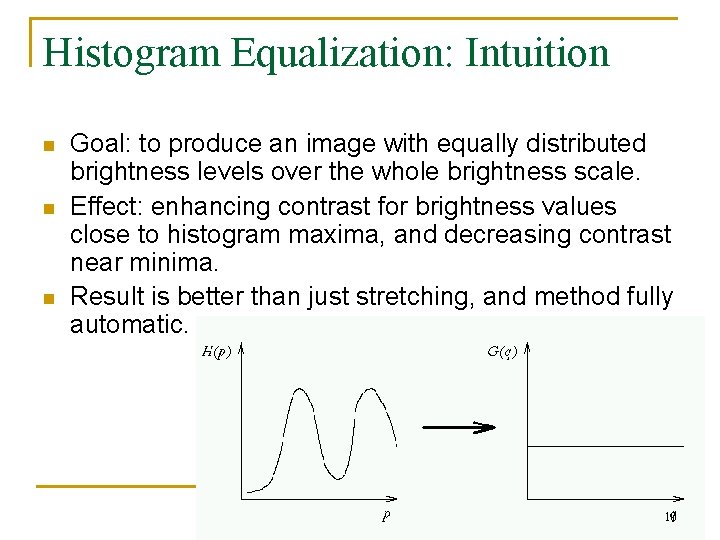
Histogram Equalization: Intuition n Goal: to produce an image with equally distributed brightness levels over the whole brightness scale. Effect: enhancing contrast for brightness values close to histogram maxima, and decreasing contrast near minima. Result is better than just stretching, and method fully automatic. 10

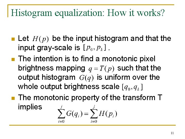
Histogram equalization: How it works? n n n Let be the input histogram and that the input gray-scale is. The intention is to find a monotonic pixel brightness mapping such that the output histogram is uniform over the whole output brightness scale The monotonic property of the transform T implies 11

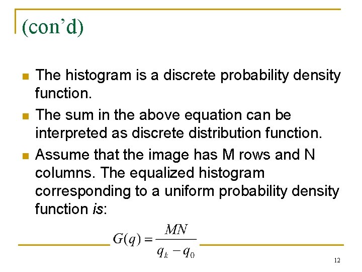
(con’d) n n n The histogram is a discrete probability density function. The sum in the above equation can be interpreted as discrete distribution function. Assume that the image has M rows and N columns. The equalized histogram corresponding to a uniform probability density function is: 12

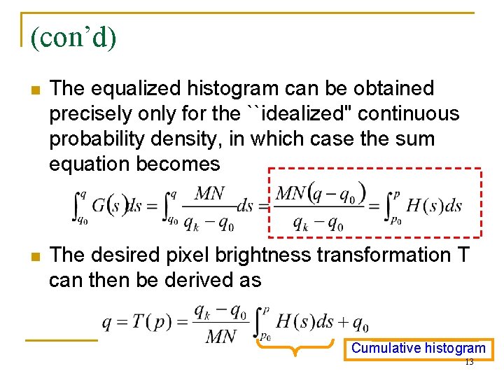
(con’d) n The equalized histogram can be obtained precisely only for the ``idealized'' continuous probability density, in which case the sum equation becomes n The desired pixel brightness transformation T can then be derived as Cumulative histogram 13

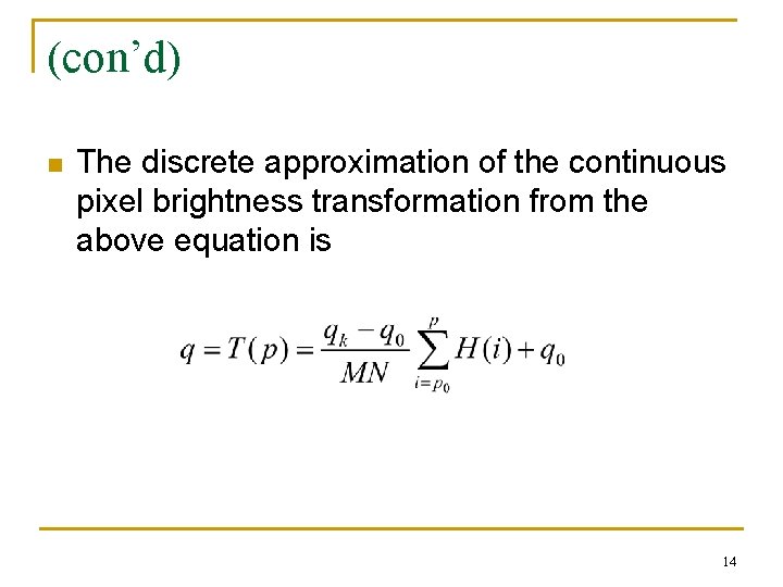
(con’d) n The discrete approximation of the continuous pixel brightness transformation from the above equation is 14

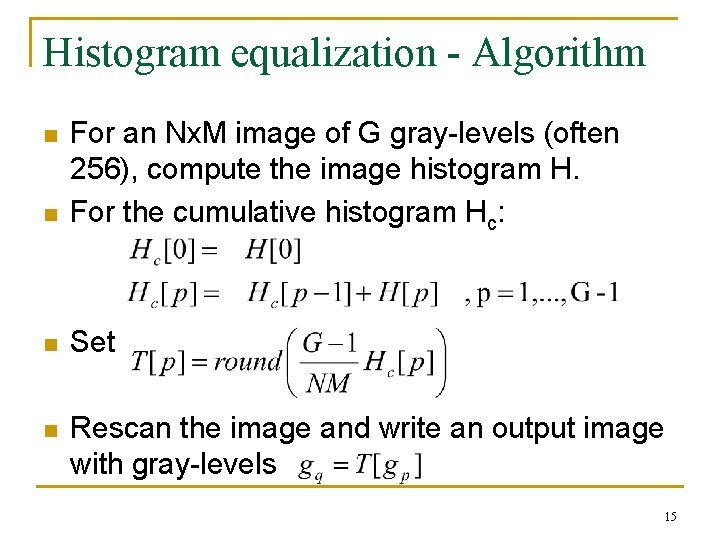
Histogram equalization - Algorithm n For an Nx. M image of G gray-levels (often 256), compute the image histogram H. For the cumulative histogram Hc: n Set n Rescan the image and write an output image with gray-levels n 15

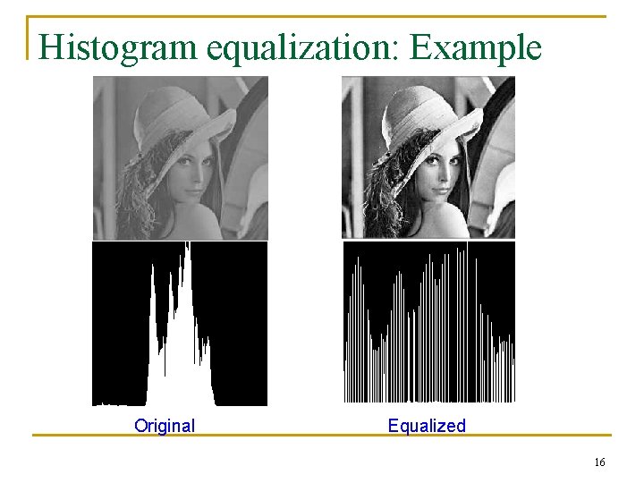
Histogram equalization: Example Original Equalized 16

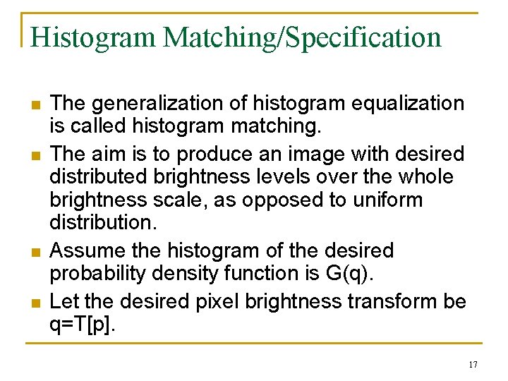
Histogram Matching/Specification n n The generalization of histogram equalization is called histogram matching. The aim is to produce an image with desired distributed brightness levels over the whole brightness scale, as opposed to uniform distribution. Assume the histogram of the desired probability density function is G(q). Let the desired pixel brightness transform be q=T[p]. 17

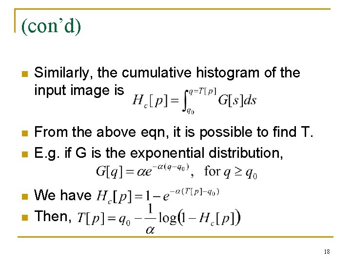
(con’d) n Similarly, the cumulative histogram of the input image is n From the above eqn, it is possible to find T. E. g. if G is the exponential distribution, n n n We have Then, 18

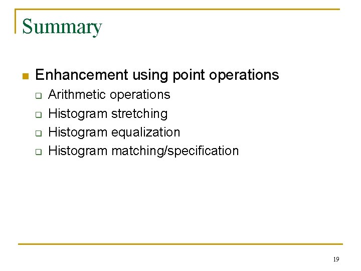
Summary n Enhancement using point operations q q Arithmetic operations Histogram stretching Histogram equalization Histogram matching/specification 19