Digital Image Processing Lecture 16 Segmentation Detection of

Digital Image Processing Lecture 16: Segmentation: Detection of Discontinuities May 2, 2005 Prof. Charlene Tsai Digital Image Processing Lecture 16

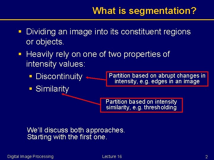
What is segmentation? § Dividing an image into its constituent regions or objects. § Heavily rely on one of two properties of intensity values: Partition based on abrupt changes in § Discontinuity intensity, e. g. edges in an image § Similarity Partition based on intensity similarity, e. g. thresholding We’ll discuss both approaches. Starting with the first one. Digital Image Processing Lecture 16 2

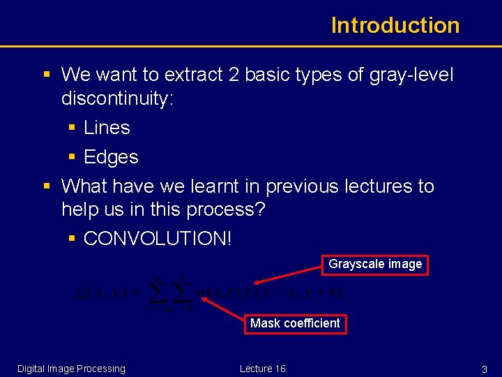
Introduction § We want to extract 2 basic types of gray-level discontinuity: § Lines § Edges § What have we learnt in previous lectures to help us in this process? § CONVOLUTION! Grayscale image Mask coefficient Digital Image Processing Lecture 16 3

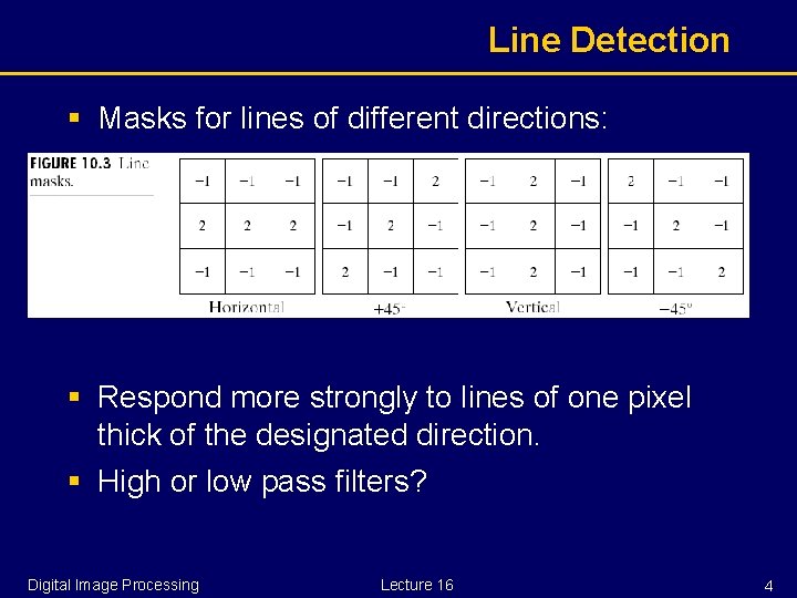
Line Detection § Masks for lines of different directions: § Respond more strongly to lines of one pixel thick of the designated direction. § High or low pass filters? Digital Image Processing Lecture 16 4

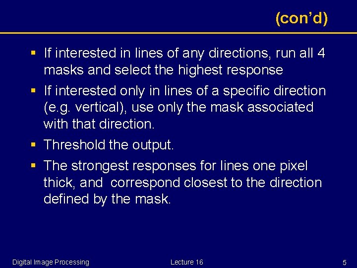
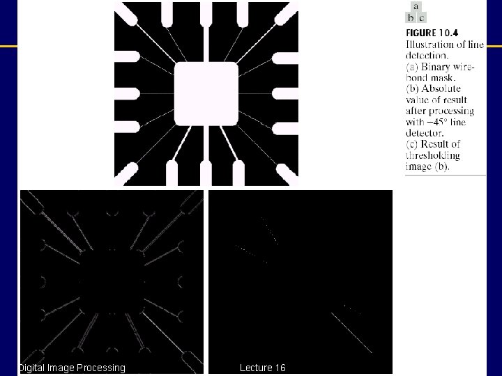
(con’d) § If interested in lines of any directions, run all 4 masks and select the highest response § If interested only in lines of a specific direction (e. g. vertical), use only the mask associated with that direction. § Threshold the output. § The strongest responses for lines one pixel thick, and correspond closest to the direction defined by the mask. Digital Image Processing Lecture 16 5

Digital Image Processing Lecture 16 6

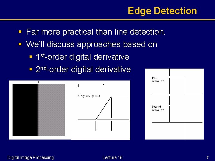
Edge Detection § Far more practical than line detection. § We’ll discuss approaches based on § 1 st-order digital derivative § 2 nd-order digital derivative Digital Image Processing Lecture 16 7

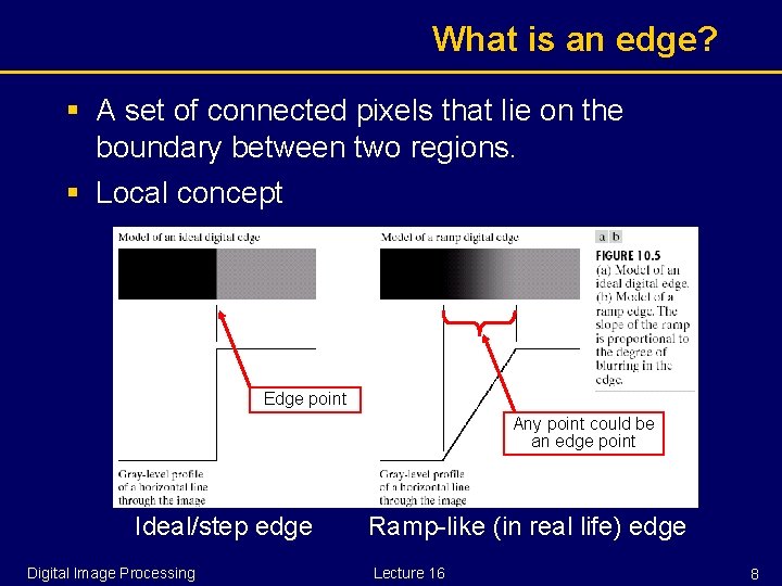
What is an edge? § A set of connected pixels that lie on the boundary between two regions. § Local concept Edge point Any point could be an edge point Ideal/step edge Digital Image Processing Ramp-like (in real life) edge Lecture 16 8

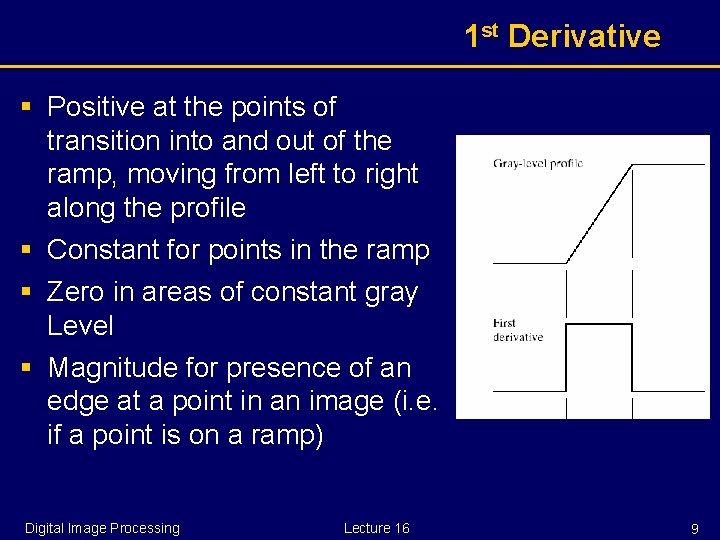
1 st Derivative § Positive at the points of transition into and out of the ramp, moving from left to right along the profile § Constant for points in the ramp § Zero in areas of constant gray Level § Magnitude for presence of an edge at a point in an image (i. e. if a point is on a ramp) Digital Image Processing Lecture 16 9

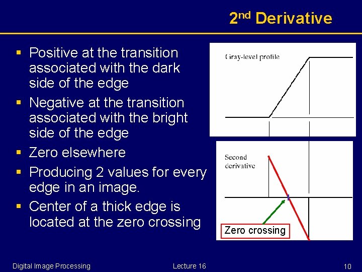
2 nd Derivative § Positive at the transition associated with the dark side of the edge § Negative at the transition associated with the bright side of the edge § Zero elsewhere § Producing 2 values for every edge in an image. § Center of a thick edge is located at the zero crossing Digital Image Processing Lecture 16 Zero crossing 10

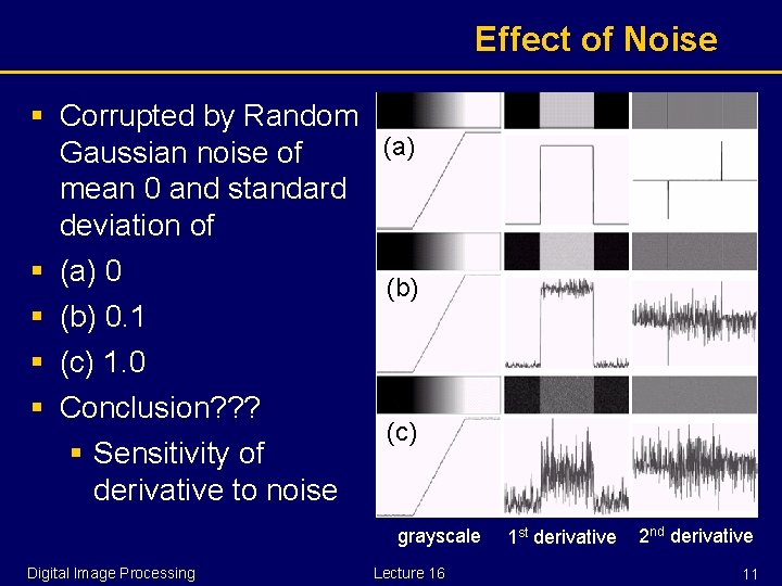
Effect of Noise § Corrupted by Random (a) Gaussian noise of mean 0 and standard deviation of § (a) 0 (b) § (b) 0. 1 § (c) 1. 0 § Conclusion? ? ? (c) § Sensitivity of derivative to noise grayscale Digital Image Processing Lecture 16 1 st derivative 2 nd derivative 11

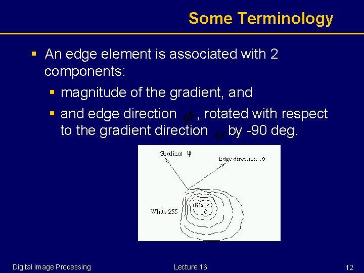
Some Terminology § An edge element is associated with 2 components: § magnitude of the gradient, and § and edge direction , rotated with respect to the gradient direction by -90 deg. Digital Image Processing Lecture 16 12

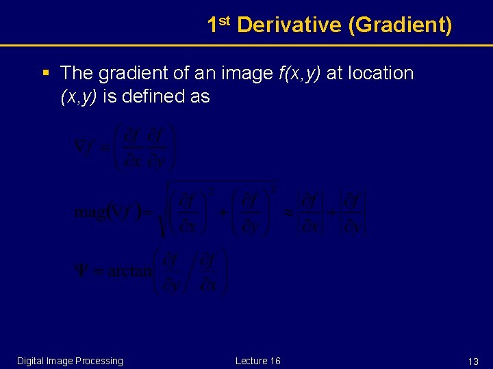
1 st Derivative (Gradient) § The gradient of an image f(x, y) at location (x, y) is defined as Digital Image Processing Lecture 16 13

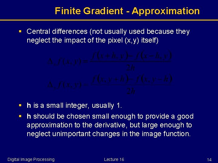
Finite Gradient - Approximation § Central differences (not usually used because they neglect the impact of the pixel (x, y) itself) § h is a small integer, usually 1. § h should be chosen small enough to provide a good approximation to the derivative, but large enough to neglect unimportant changes in the image function. Digital Image Processing Lecture 16 14

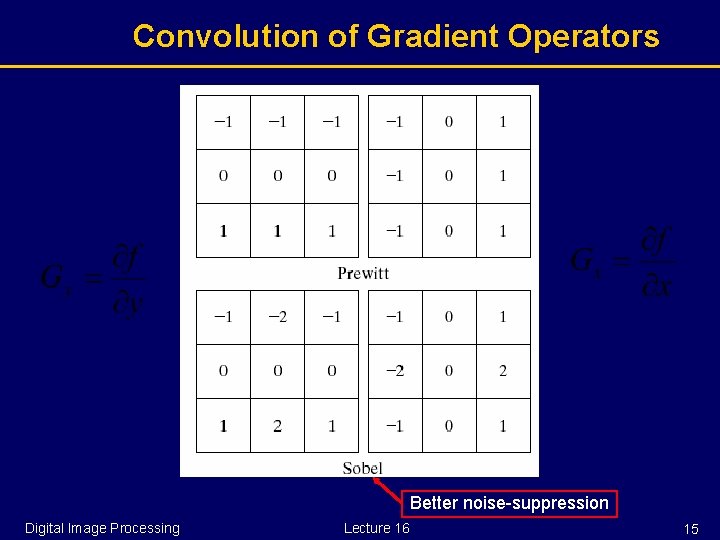
Convolution of Gradient Operators Better noise-suppression Digital Image Processing Lecture 16 15

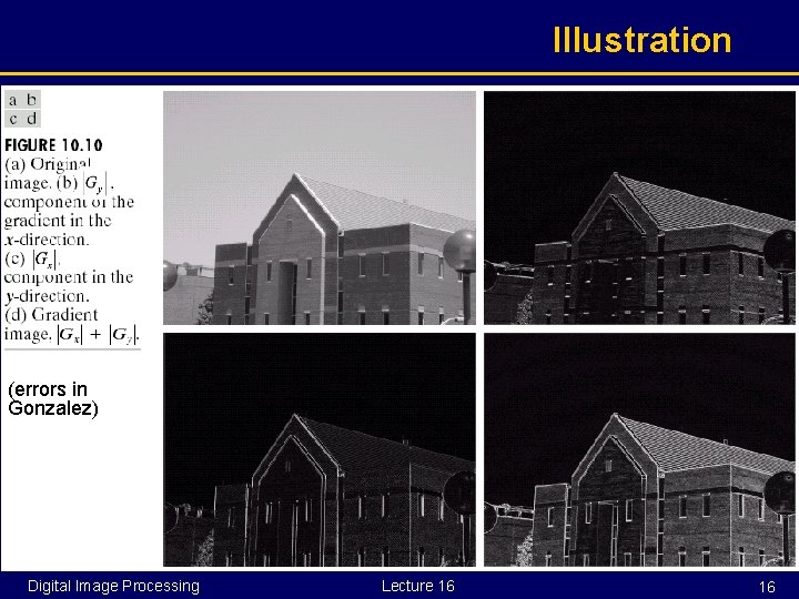
Illustration (errors in Gonzalez) Digital Image Processing Lecture 16 16

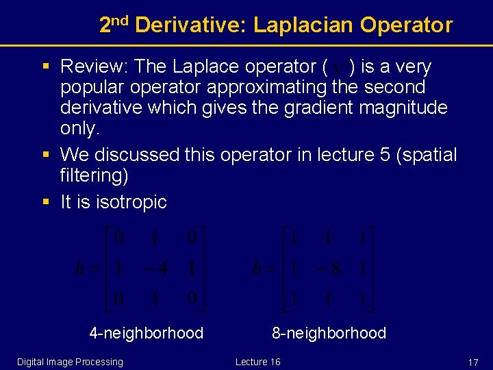
2 nd Derivative: Laplacian Operator § Review: The Laplace operator ( ) is a very popular operator approximating the second derivative which gives the gradient magnitude only. § We discussed this operator in lecture 5 (spatial filtering) § It is isotropic 4 -neighborhood Digital Image Processing 8 -neighborhood Lecture 16 17

Issues with Laplacian § Problems: § Unacceptably sensitive to noise § Magnitude of Laplacian results in double edges § Does not provide gradient § Fixes: § Smoothing § Using zero-crossing for edge location § Not for gradient direction, but for establishing whether a pixel is on the dark or light side of and edge Digital Image Processing Lecture 16 18

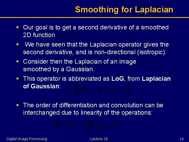
Smoothing for Laplacian § Our goal is to get a second derivative of a smoothed 2 D function § We have seen that the Laplacian operator gives the second derivative, and is non-directional (isotropic). § Consider then the Laplacian of an image smoothed by a Gaussian. § This operator is abbreviated as Lo. G, from Laplacian of Gaussian: § The order of differentiation and convolution can be interchanged due to linearity of the operations: Digital Image Processing Lecture 16 19

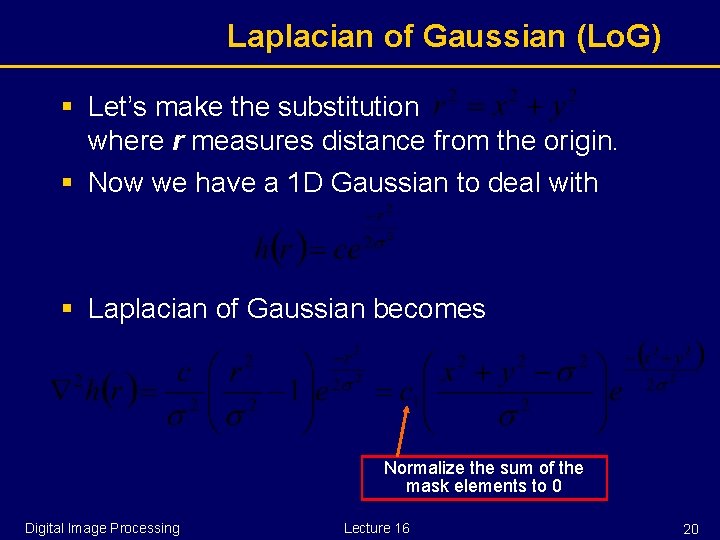
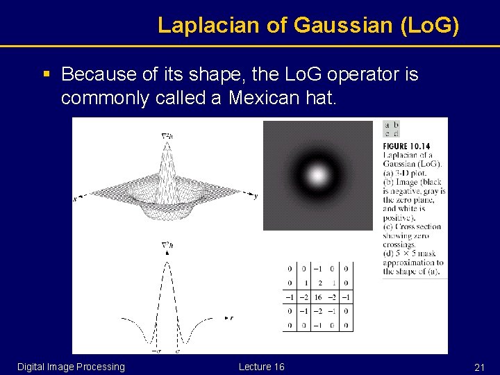
Laplacian of Gaussian (Lo. G) § Let’s make the substitution where r measures distance from the origin. § Now we have a 1 D Gaussian to deal with § Laplacian of Gaussian becomes Normalize the sum of the mask elements to 0 Digital Image Processing Lecture 16 20

Laplacian of Gaussian (Lo. G) § Because of its shape, the Lo. G operator is commonly called a Mexican hat. Digital Image Processing Lecture 16 21

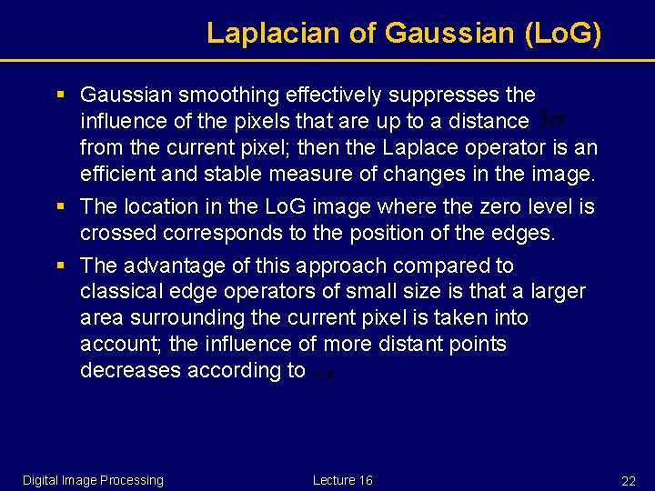
Laplacian of Gaussian (Lo. G) § Gaussian smoothing effectively suppresses the influence of the pixels that are up to a distance from the current pixel; then the Laplace operator is an efficient and stable measure of changes in the image. § The location in the Lo. G image where the zero level is crossed corresponds to the position of the edges. § The advantage of this approach compared to classical edge operators of small size is that a larger area surrounding the current pixel is taken into account; the influence of more distant points decreases according to Digital Image Processing Lecture 16 22

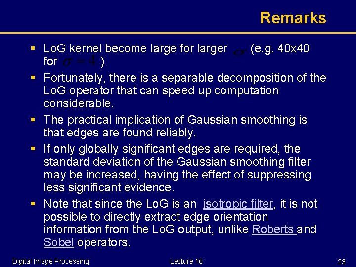
Remarks § Lo. G kernel become large for larger (e. g. 40 x 40 for ) § Fortunately, there is a separable decomposition of the Lo. G operator that can speed up computation considerable. § The practical implication of Gaussian smoothing is that edges are found reliably. § If only globally significant edges are required, the standard deviation of the Gaussian smoothing filter may be increased, having the effect of suppressing less significant evidence. § Note that since the Lo. G is an isotropic filter, it is not possible to directly extract edge orientation information from the Lo. G output, unlike Roberts and Sobel operators. Digital Image Processing Lecture 16 23

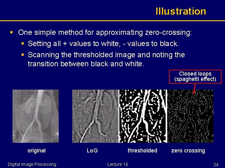
Illustration § One simple method for approximating zero-crossing: § Setting all + values to white, - values to black. § Scanning the thresholded image and noting the transition between black and white. Closed loops (spaghetti effect) original Digital Image Processing Lo. G thresholded Lecture 16 zero crossing 24

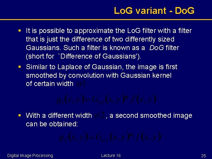
Lo. G variant - Do. G § It is possible to approximate the Lo. G filter with a filter that is just the difference of two differently sized Gaussians. Such a filter is known as a Do. G filter (short for `Difference of Gaussians'). § Similar to Laplace of Gaussian, the image is first smoothed by convolution with Gaussian kernel of certain width § With a different width can be obtained: Digital Image Processing , a second smoothed image Lecture 16 25

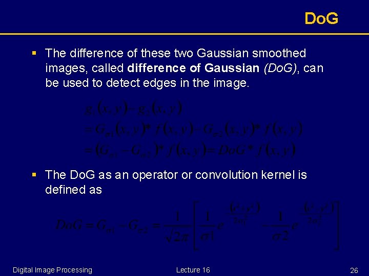
Do. G § The difference of these two Gaussian smoothed images, called difference of Gaussian (Do. G), can be used to detect edges in the image. § The Do. G as an operator or convolution kernel is defined as Digital Image Processing Lecture 16 26

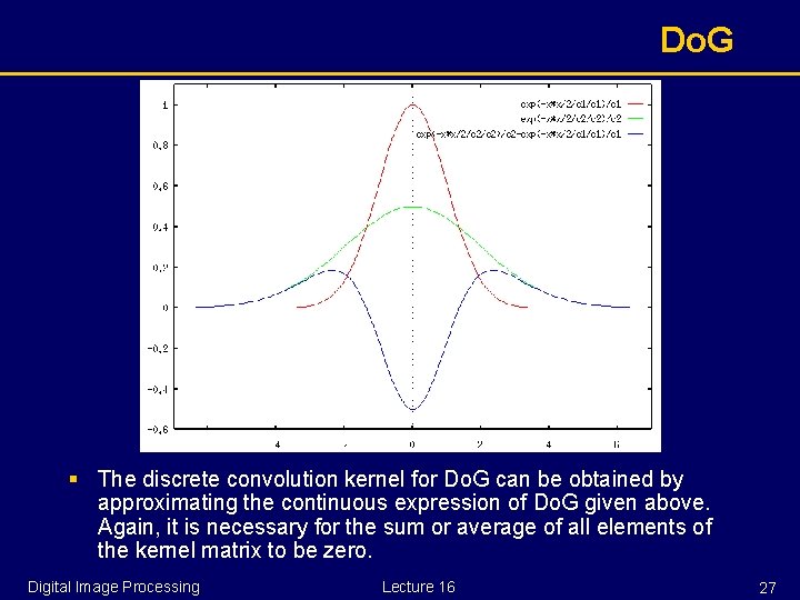
Do. G § The discrete convolution kernel for Do. G can be obtained by approximating the continuous expression of Do. G given above. Again, it is necessary for the sum or average of all elements of the kernel matrix to be zero. Digital Image Processing Lecture 16 27

Summary § Line detection § Edge detection based on § First derivative § Provides gradient information § 2 nd derivative using zero-crossing § Indicates dark/bright side of an edge Digital Image Processing Lecture 16 28