Digital Image Processing Image Enhancement in the Spatial

Digital Image Processing Image Enhancement in the Spatial Domain 1

Image Enhancement n To process an image so that the result is more suitable than the original image for a specific application. n Spatial domain methods and frequency domain methods. 2

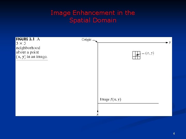
Spatial Domain Methods n Procedures that operate directly on the aggregate of pixels composing an image n. A neighborhood about (x, y) is defined by using a square (or rectangular) subimage area centered at (x, y). 3

Image Enhancement in the Spatial Domain 4

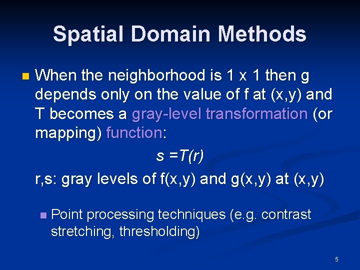
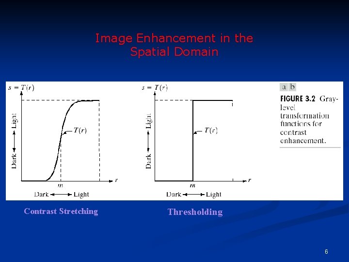
Spatial Domain Methods n When the neighborhood is 1 x 1 then g depends only on the value of f at (x, y) and T becomes a gray-level transformation (or mapping) function: s =T(r) r, s: gray levels of f(x, y) and g(x, y) at (x, y) n Point processing techniques (e. g. contrast stretching, thresholding) 5

Image Enhancement in the Spatial Domain Contrast Stretching Thresholding 6

Spatial Domain Methods n Mask processing or filtering: when the values of f in a predefined neighborhood of (x, y) determine the value of g at (x, y). n Through the use of masks (or kernels, templates, or windows, or filters). 7

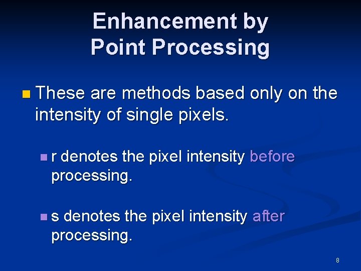
Enhancement by Point Processing n These are methods based only on the intensity of single pixels. nr denotes the pixel intensity before processing. ns denotes the pixel intensity after processing. 8

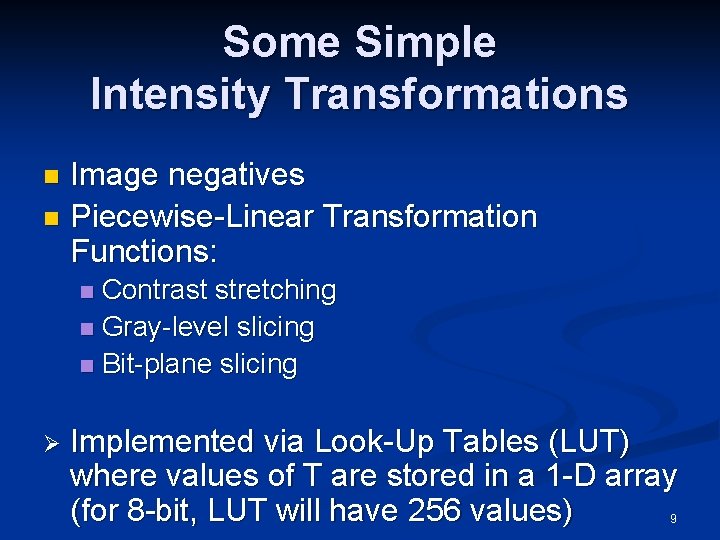
Some Simple Intensity Transformations Image negatives n Piecewise-Linear Transformation Functions: n Contrast stretching n Gray-level slicing n Bit-plane slicing n Ø Implemented via Look-Up Tables (LUT) where values of T are stored in a 1 -D array (for 8 -bit, LUT will have 256 values) 9

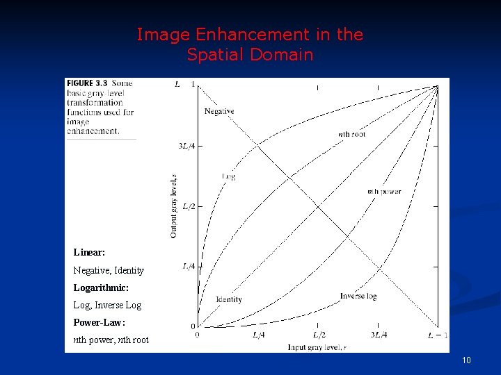
Image Enhancement in the Spatial Domain Linear: Negative, Identity Logarithmic: Log, Inverse Log Power-Law: nth power, nth root 10

Image Negatives n Are obtained by using the transformation function s=T(r). [0, L-1] the range of gray levels S= (L-1)-r 11

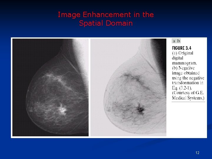
Image Enhancement in the Spatial Domain 12

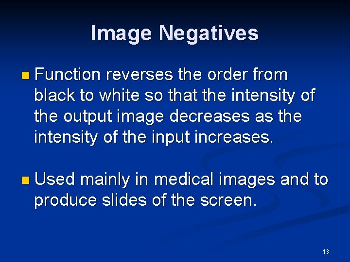
Image Negatives n Function reverses the order from black to white so that the intensity of the output image decreases as the intensity of the input increases. n Used mainly in medical images and to produce slides of the screen. 13

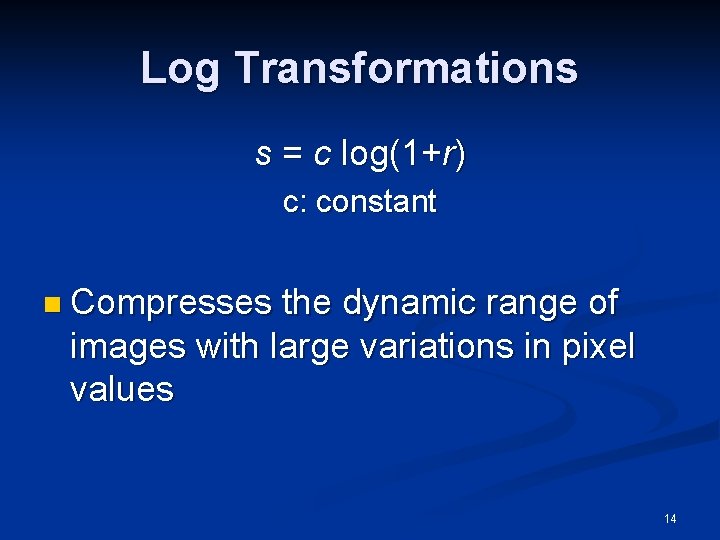
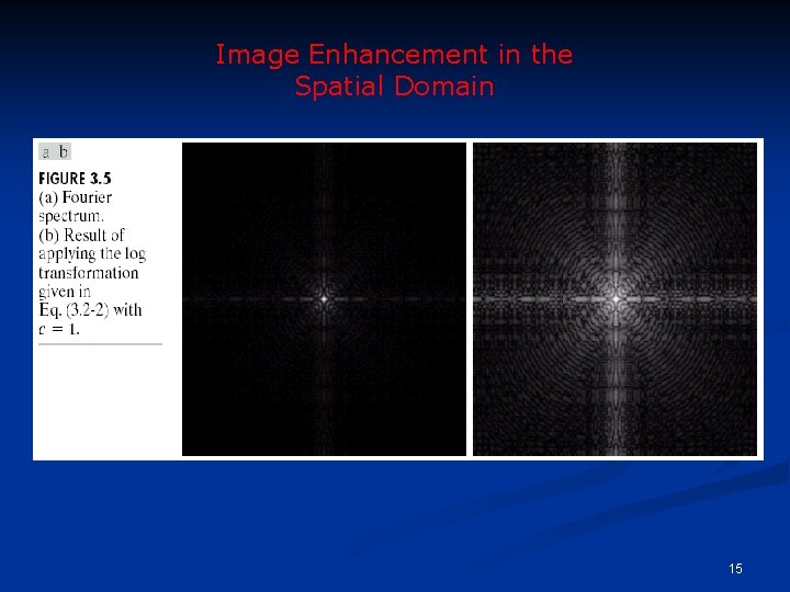
Log Transformations s = c log(1+r) c: constant n Compresses the dynamic range of images with large variations in pixel values 14

Image Enhancement in the Spatial Domain 15

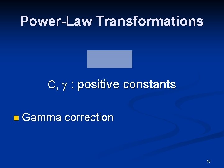
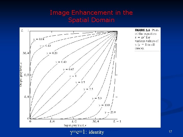
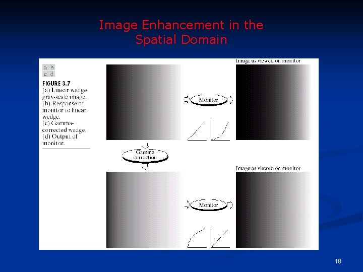
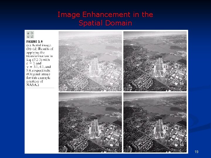
Power-Law Transformations C, : positive constants n Gamma correction 16

Image Enhancement in the Spatial Domain =c=1: identity 17

Image Enhancement in the Spatial Domain 18

Image Enhancement in the Spatial Domain 19

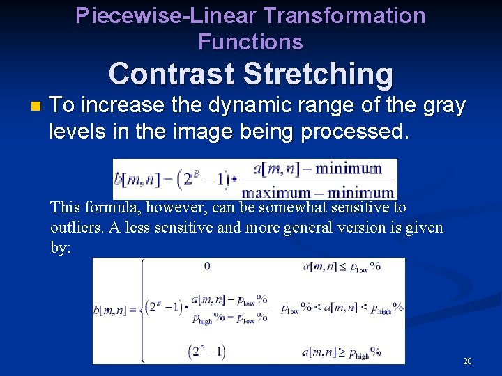
Piecewise-Linear Transformation Functions Contrast Stretching n To increase the dynamic range of the gray levels in the image being processed. This formula, however, can be somewhat sensitive to outliers. A less sensitive and more general version is given by: 20

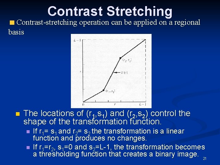
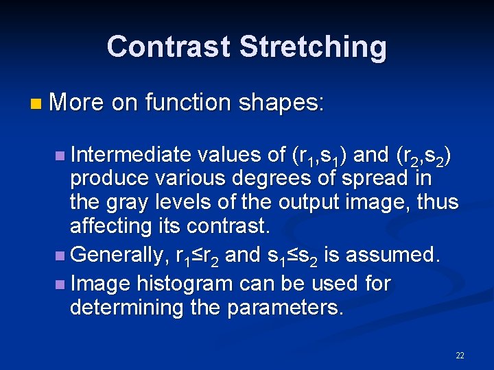
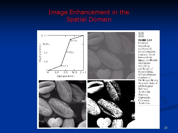
Contrast Stretching Contrast-stretching operation can be applied on a regional basis n The locations of (r 1, s 1) and (r 2, s 2) control the shape of the transformation function. n n If r 1= s 1 and r 2= s 2 the transformation is a linear function and produces no changes. If r 1=r 2, s 1=0 and s 2=L-1, the transformation becomes a thresholding function that creates a binary image. 21

Contrast Stretching n More on function shapes: n Intermediate values of (r 1, s 1) and (r 2, s 2) produce various degrees of spread in the gray levels of the output image, thus affecting its contrast. n Generally, r 1≤r 2 and s 1≤s 2 is assumed. n Image histogram can be used for determining the parameters. 22

Image Enhancement in the Spatial Domain 23

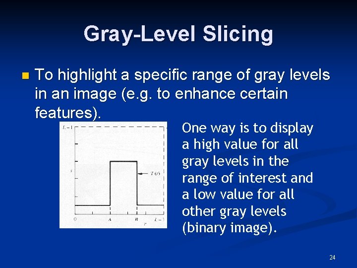
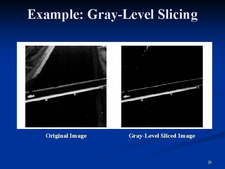
Gray-Level Slicing n To highlight a specific range of gray levels in an image (e. g. to enhance certain features). One way is to display a high value for all gray levels in the range of interest and a low value for all other gray levels (binary image). 24

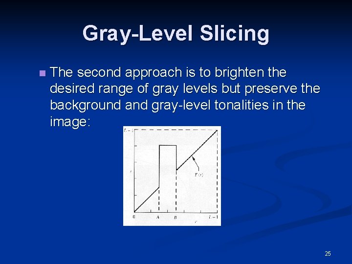
Gray-Level Slicing n The second approach is to brighten the desired range of gray levels but preserve the background and gray-level tonalities in the image: 25

Example: Gray-Level Slicing Original Image Gray-Level Sliced Image 26

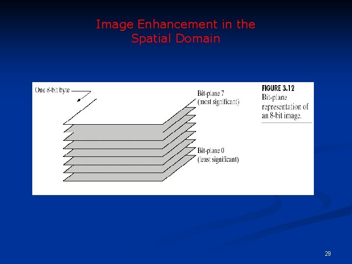
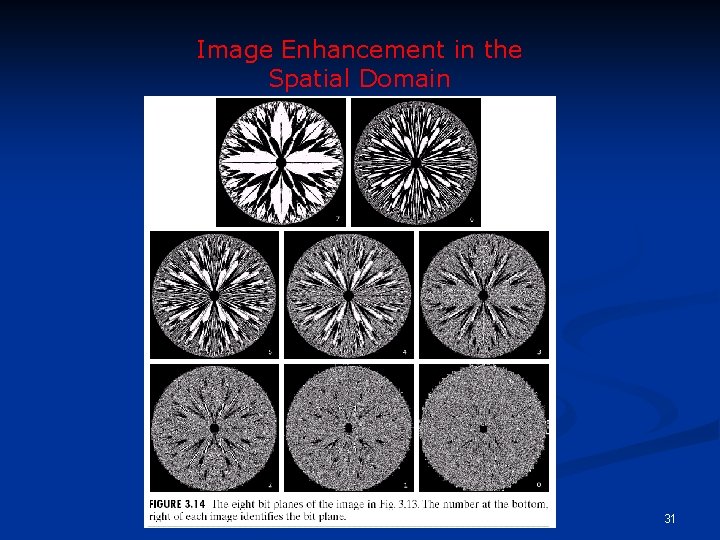
Bit-Plane Slicing n To highlight the contribution made to the total image appearance by specific bits. n i. e. Assuming that each pixel is represented by 8 bits, the image is composed of 8 1 -bit planes. n Plane 0 contains the least significant bit and plane 7 contains the most significant bit. 27

Bit-Plane Slicing n More on bit planes: n Only the higher order bits (top four) contain visually significant data. The other bit planes contribute the more subtle details. n Plane 7 corresponds exactly with an image thresholded at gray level 128. 28

Image Enhancement in the Spatial Domain 29

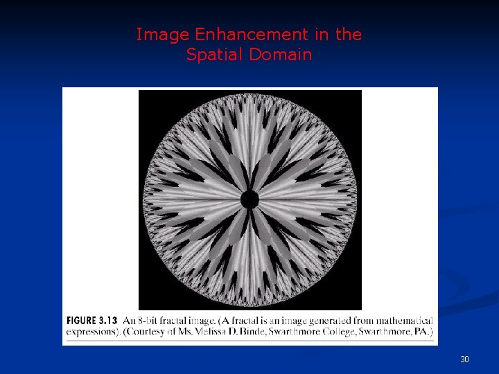
Image Enhancement in the Spatial Domain 30

Image Enhancement in the Spatial Domain 31

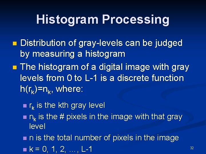
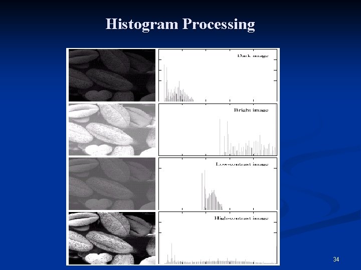
Histogram Processing Distribution of gray-levels can be judged by measuring a histogram n The histogram of a digital image with gray levels from 0 to L-1 is a discrete function h(rk)=nk, where: n n rk is the kth gray level n nk is the # pixels in the image with that gray level n n is the total number of pixels in the image n k = 0, 1, 2, …, L-1 32

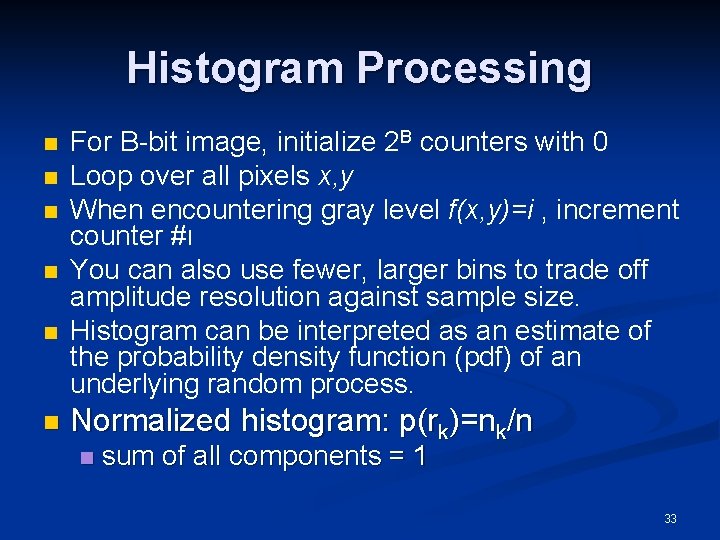
Histogram Processing n n n For B-bit image, initialize 2 B counters with 0 Loop over all pixels x, y When encountering gray level f(x, y)=i , increment counter #ι You can also use fewer, larger bins to trade off amplitude resolution against sample size. Histogram can be interpreted as an estimate of the probability density function (pdf) of an underlying random process. Normalized histogram: p(rk)=nk/n n sum of all components = 1 33

Histogram Processing 34

Histogram Processing n The shape of the histogram of an image does provide useful info about the possibility for contrast enhancement. n Types of processing: n n n Histogram equalization Histogram matching (specification) Local enhancement 35

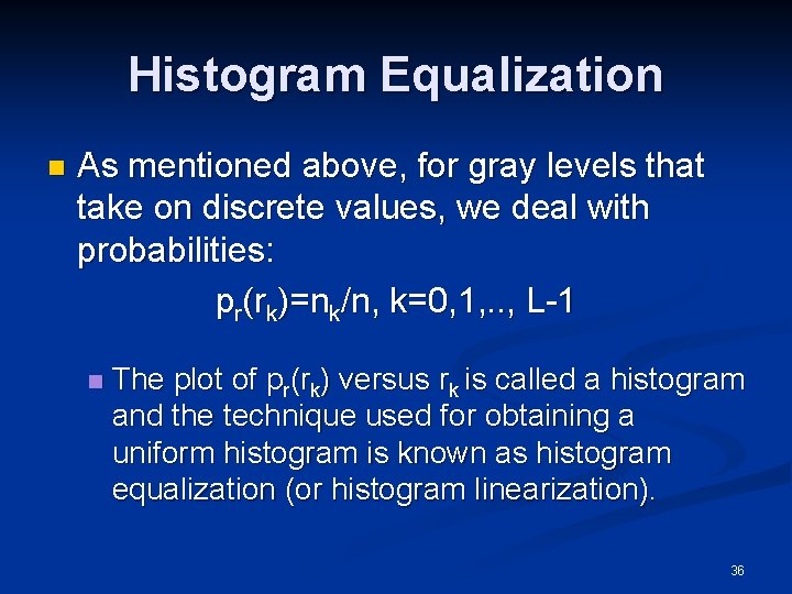
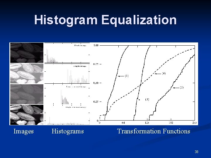
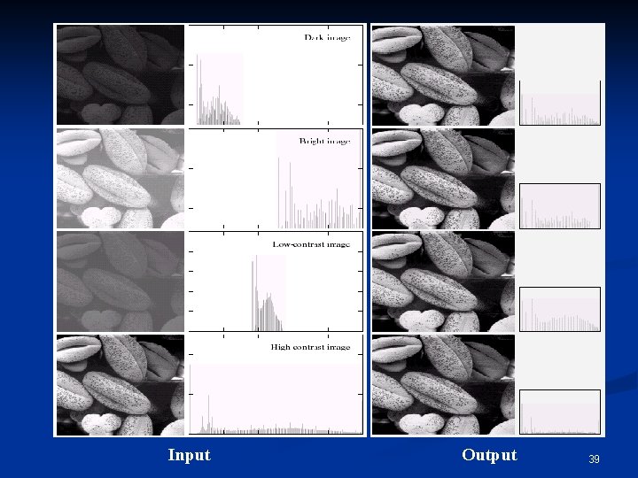
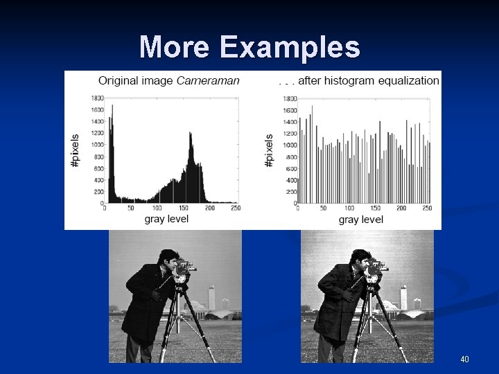
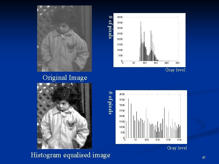
Histogram Equalization n As mentioned above, for gray levels that take on discrete values, we deal with probabilities: pr(rk)=nk/n, k=0, 1, . . , L-1 n The plot of pr(rk) versus rk is called a histogram and the technique used for obtaining a uniform histogram is known as histogram equalization (or histogram linearization). 36

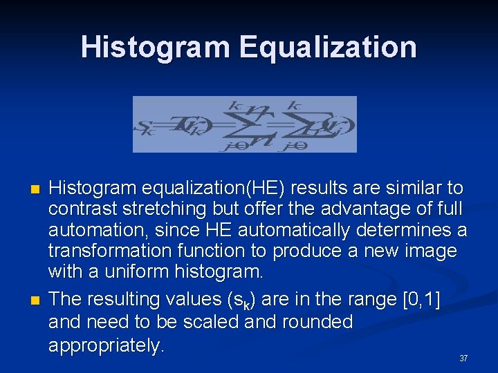
Histogram Equalization n n Histogram equalization(HE) results are similar to contrast stretching but offer the advantage of full automation, since HE automatically determines a transformation function to produce a new image with a uniform histogram. The resulting values (sk) are in the range [0, 1] and need to be scaled and rounded appropriately. 37

Histogram Equalization Images Histograms Transformation Functions 38

Input Output 39

More Examples 40

# of pixels Gray level Original Image # of pixels Gray level Histogram equalised image 41

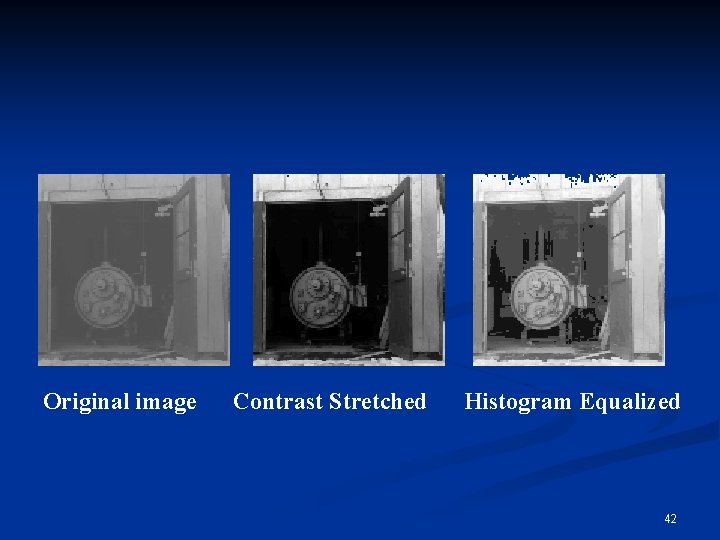
Original image Contrast Stretched Histogram Equalized 42

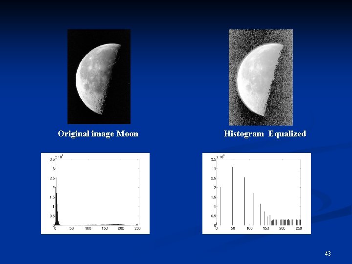
Original image Moon Histogram Equalized 43

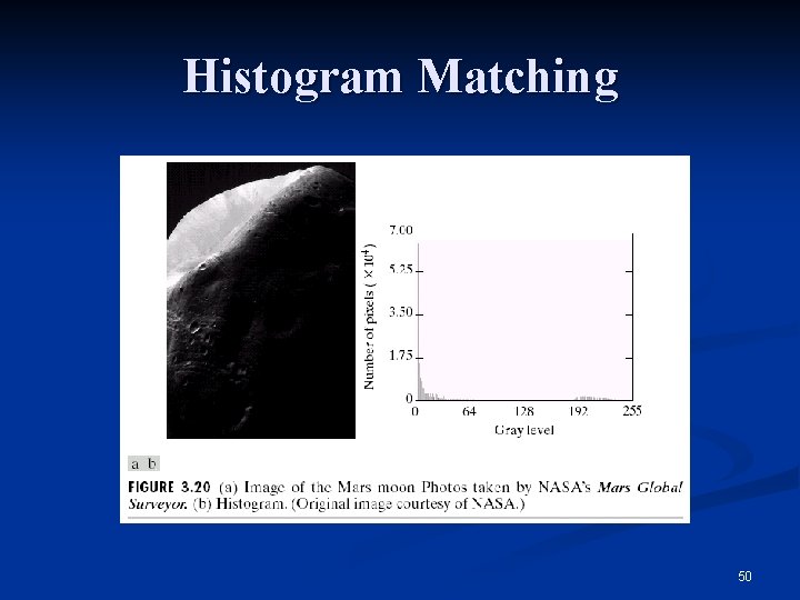
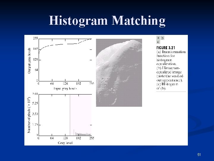
Histogram Matching (or Specification) n Histogram equalization does not allow interactive image enhancement and generates only one result: an approximation to a uniform histogram. n Sometimes though, we need to be able to specify particular histogram shapes capable of highlighting certain gray-level ranges. 44

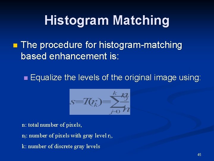
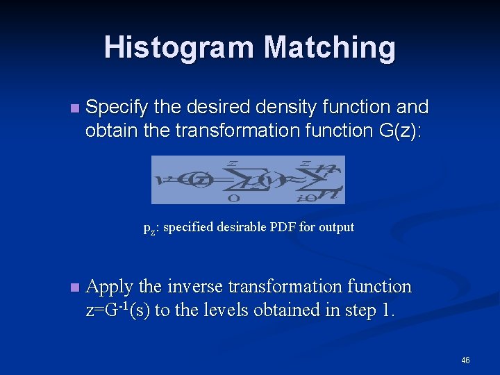
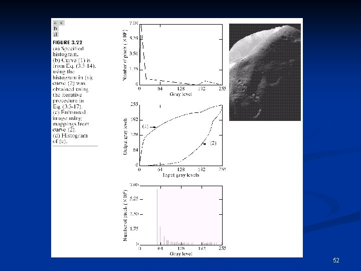
Histogram Matching n The procedure for histogram-matching based enhancement is: n Equalize the levels of the original image using: n: total number of pixels, nj: number of pixels with gray level rj, k: number of discrete gray levels 45

Histogram Matching n Specify the desired density function and obtain the transformation function G(z): pz: specified desirable PDF for output n Apply the inverse transformation function z=G-1(s) to the levels obtained in step 1. 46

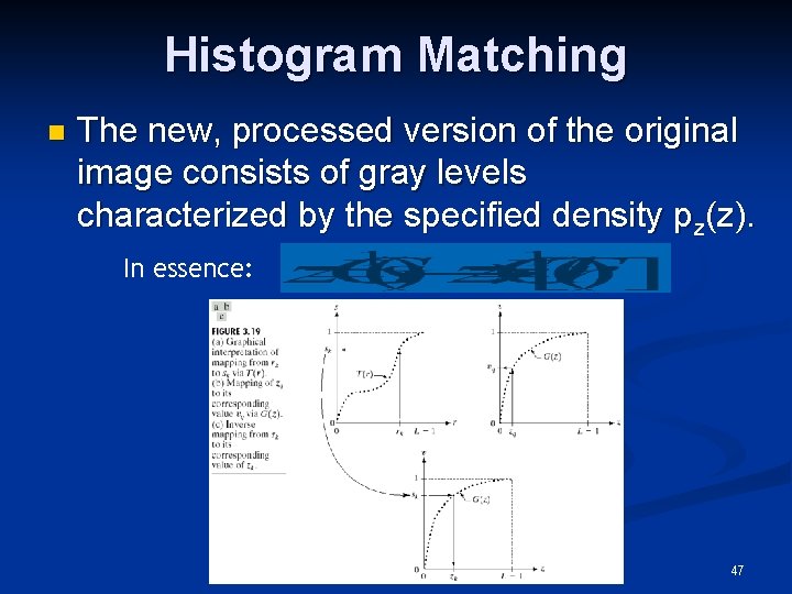
Histogram Matching n The new, processed version of the original image consists of gray levels characterized by the specified density pz(z). In essence: 47

Histogram Matching n The principal difficulty in applying the histogram matching method to image enhancement lies in being able to construct a meaningful histogram. So… 48

Histogram Matching n Either a particular probability density function (such as a Gaussian density) is specified and then a histogram is formed by digitizing the given function, n Or a histogram shape is specified on a graphic device and then is fed into the processor executing the histogram matching algorithm. 49

Histogram Matching 50

Histogram Matching 51

52

Local Enhancement n When it is necessary to enhance details over smaller areas n To devise transformation functions based on the gray-level distribution in the neighborhood of every pixel 53

Local Enhancement n The procedure is: n Define a square (or rectangular) neighborhood and move the center of this area from pixel to pixel. n At each location, the histogram of the points in the neighborhood is computed and either a histogram equalization or histogram matching transformation function is obtained. n This function is finally used to map the gray level of the pixel centered in the neighborhood. n The center is then moved to an adjacent pixel 54 location and the procedure is repeated.

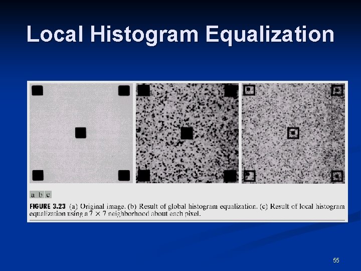
Local Histogram Equalization 55

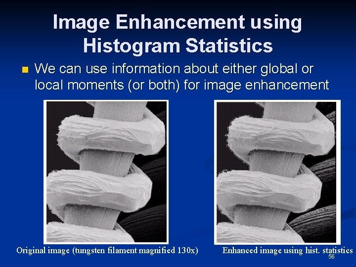
Image Enhancement using Histogram Statistics n We can use information about either global or local moments (or both) for image enhancement Original image (tungsten filament magnified 130 x) Enhanced image using hist. statistics 56

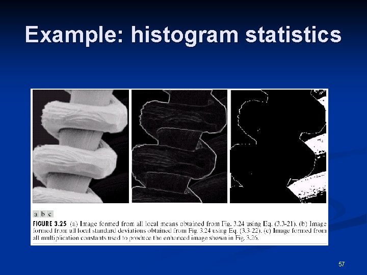
Example: histogram statistics 57

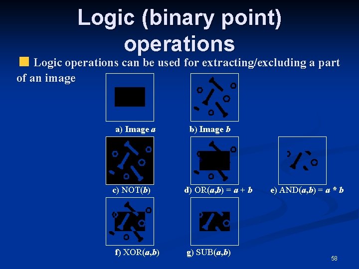
Logic (binary point) operations Logic operations can be used for extracting/excluding a part of an image a) Image a c) NOT(b) f) XOR(a, b) b) Image b d) OR(a, b) = a + b g) SUB(a, b) e) AND(a, b) = a * b 58

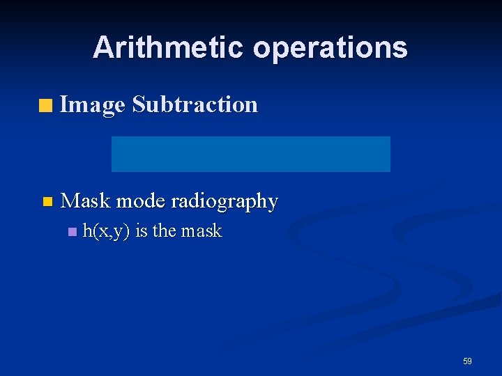
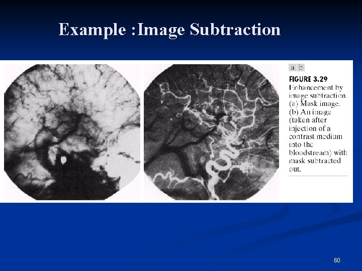
Arithmetic operations Image Subtraction n Mask mode radiography n h(x, y) is the mask 59

Example : Image Subtraction 60

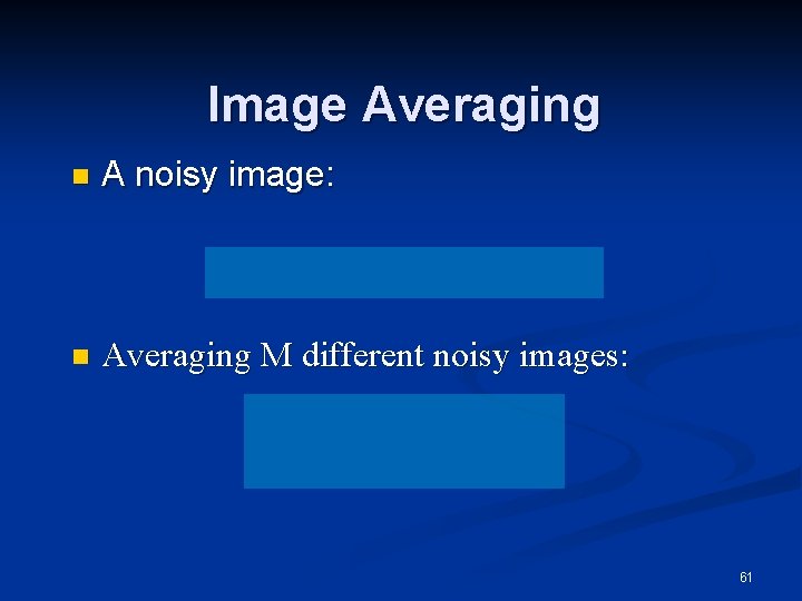
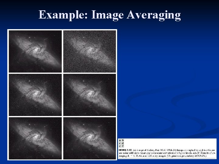
Image Averaging n A noisy image: n Averaging M different noisy images: 61

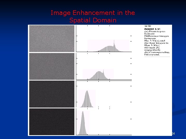
Image Averaging n As M increases, the variability of the pixel values at each location decreases. n n This means that g(x, y) approaches f(x, y) as the number of noisy images used in the averaging process increases. Registering of the images is necessary to avoid blurring in the output image. 62

Example: Image Averaging 63

Image Enhancement in the Spatial Domain 64

Spatial Filtering n Use of spatial masks for image processing (spatial filters) n Linear and nonlinear filters n Low-pass filters eliminate or attenuate high frequency components in the frequency domain (sharp image details), and result in image blurring. 65

Spatial Filtering n High-pass filters attenuate or eliminate lowfrequency components (resulting in sharpening edges and other sharp details). n Band-pass filters keep/remove selected frequency regions between low and high frequencies (for image restoration, not enhancement). 66

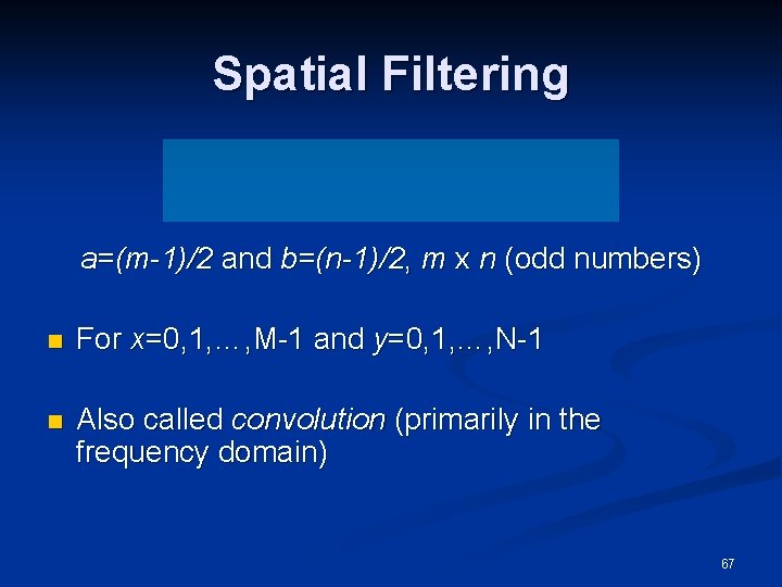
Spatial Filtering a=(m-1)/2 and b=(n-1)/2, m x n (odd numbers) n For x=0, 1, …, M-1 and y=0, 1, …, N-1 n Also called convolution (primarily in the frequency domain) 67

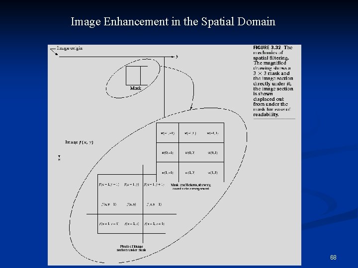
Image Enhancement in the Spatial Domain 68

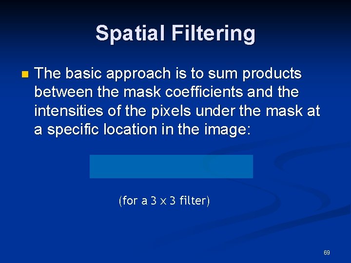
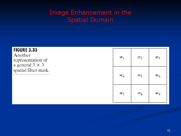
Spatial Filtering n The basic approach is to sum products between the mask coefficients and the intensities of the pixels under the mask at a specific location in the image: (for a 3 x 3 filter) 69

Image Enhancement in the Spatial Domain 70

Spatial Filtering n Non-linear filters also use pixel neighborhoods but do not explicitly use coefficients n e. g. noise reduction by median gray-level value computation in the neighborhood of the filter 71

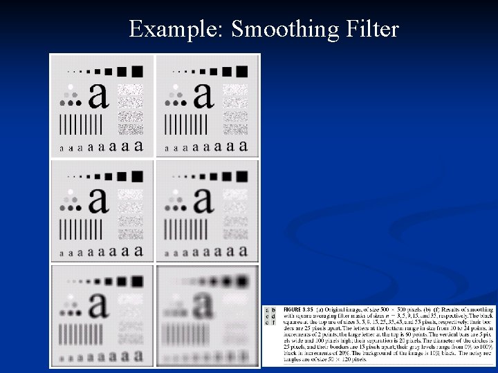
Smoothing Filters n Smoothing aims to suppress noise or other small fluctuations in the image n equivalent to the suppression of high frequencies in the frequency domain. n Used for blurring (removal of small details prior to large object extraction, bridging small gaps in lines) and noise reduction. n Unfortunately, smoothing also blurs all sharp edges that bear important information about the image. 72

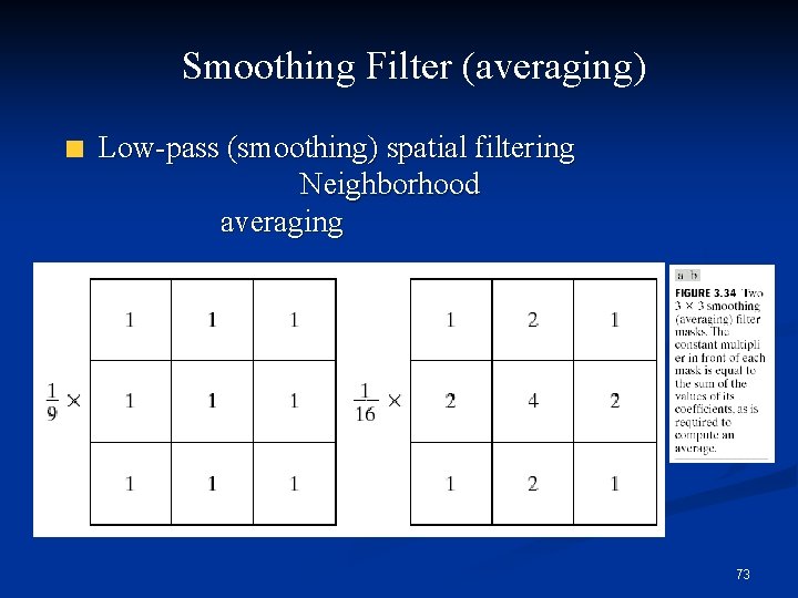
Smoothing Filter (averaging) Low-pass (smoothing) spatial filtering Neighborhood averaging 73

Example: Smoothing Filter 74

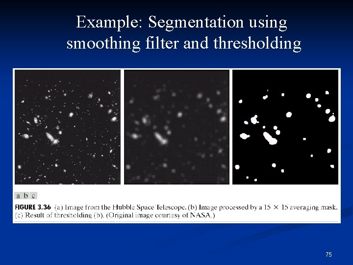
Example: Segmentation using smoothing filter and thresholding 75

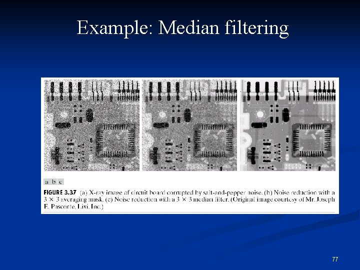
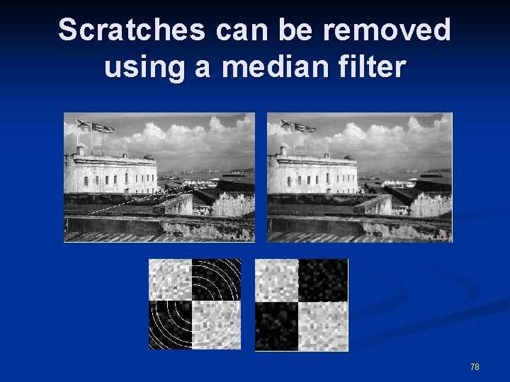
Smoothing Filters n Median filtering (nonlinear) n Used primarily for noise reduction (eliminates isolated spikes) n The gray level of each pixel is replaced by the median of the gray levels in the neighborhood of that pixel (instead of by the average as before). 76

Example: Median filtering 77

Scratches can be removed using a median filter 78

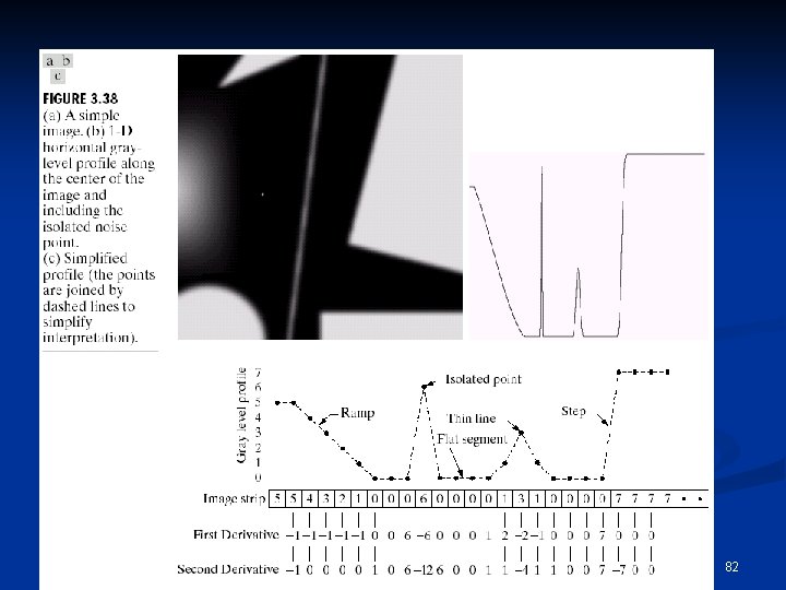
Sharpening Filters n To highlight fine detail or to enhance blurred detail. smoothing ~ integration n sharpening ~ differentiation n n Categories of sharpening filters: Derivative operators n Basic highpass spatial filtering n High-boost filtering n 79

Derivative Filters n Averaging is analogous to integration and causes blurring, so differentiation is expected to have opposite results and sharpen an image. 80

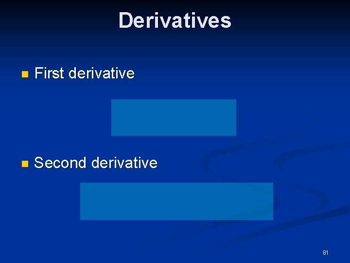
Derivatives n First derivative n Second derivative 81

82

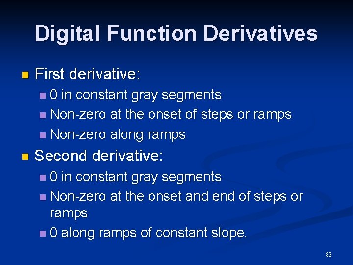
Digital Function Derivatives n First derivative: 0 in constant gray segments n Non-zero at the onset of steps or ramps n Non-zero along ramps n n Second derivative: 0 in constant gray segments n Non-zero at the onset and end of steps or ramps n 0 along ramps of constant slope. n 83

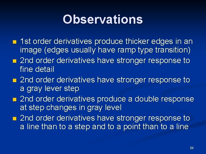
Observations n n n 1 st order derivatives produce thicker edges in an image (edges usually have ramp type transition) 2 nd order derivatives have stronger response to fine detail 2 nd order derivatives have stronger response to a gray lever step 2 nd order derivatives produce a double response at step changes in gray level 2 nd order derivatives have stronger response to a line than to a step and to a point than to a line 84

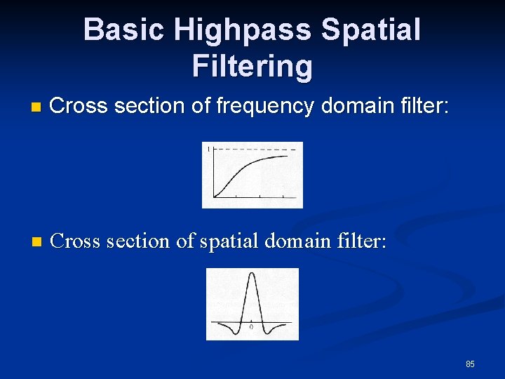
Basic Highpass Spatial Filtering n Cross section of frequency domain filter: n Cross section of spatial domain filter: 85

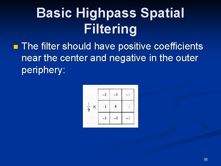
Basic Highpass Spatial Filtering n The filter should have positive coefficients near the center and negative in the outer periphery: 86

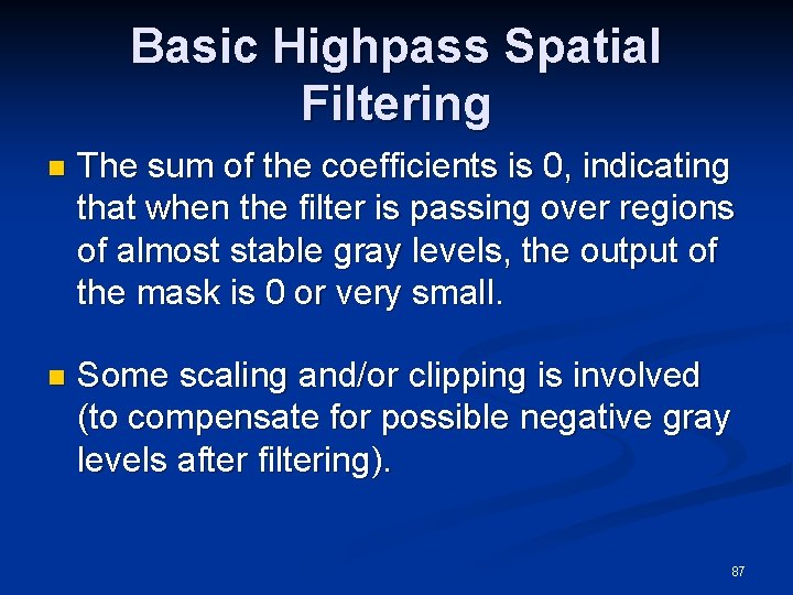
Basic Highpass Spatial Filtering n The sum of the coefficients is 0, indicating that when the filter is passing over regions of almost stable gray levels, the output of the mask is 0 or very small. n Some scaling and/or clipping is involved (to compensate for possible negative gray levels after filtering). 87

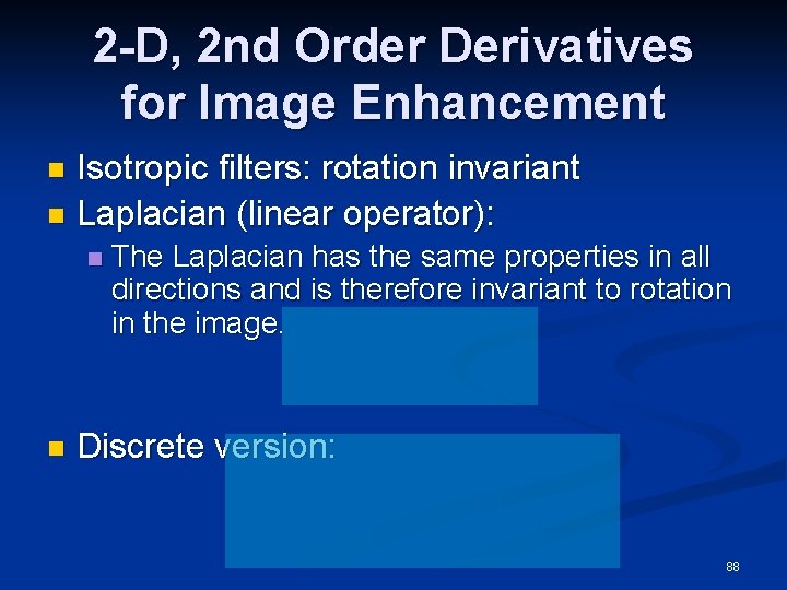
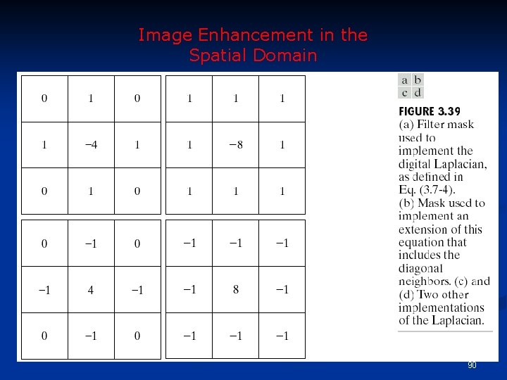
2 -D, 2 nd Order Derivatives for Image Enhancement Isotropic filters: rotation invariant n Laplacian (linear operator): n n n The Laplacian has the same properties in all directions and is therefore invariant to rotation in the image. Discrete version: 88

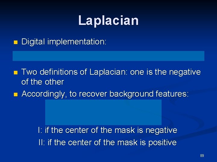
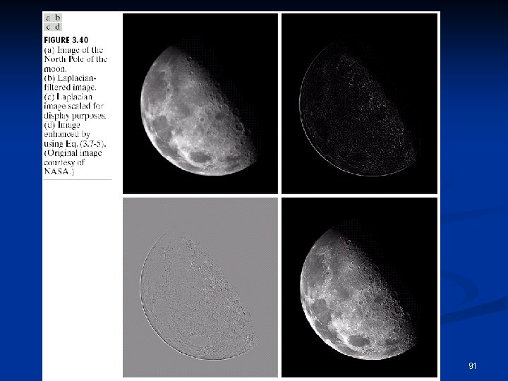
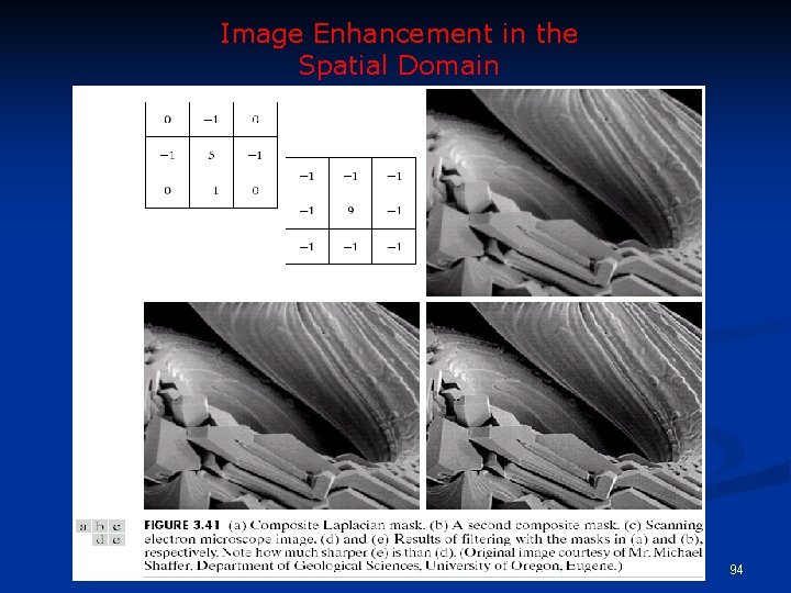
Laplacian n Digital implementation: n Two definitions of Laplacian: one is the negative of the other Accordingly, to recover background features: n I: if the center of the mask is negative II: if the center of the mask is positive 89

Image Enhancement in the Spatial Domain 90

91

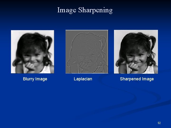
Image Sharpening Blurry Image Laplacian Sharpened Image 92

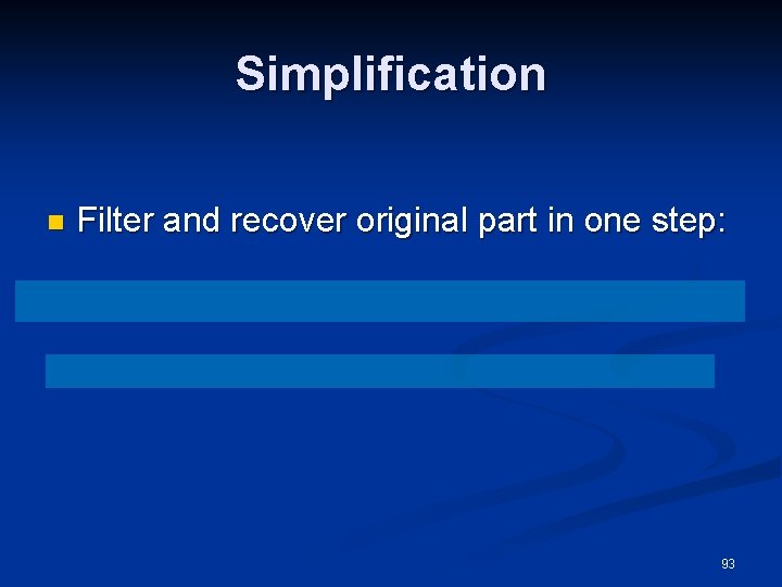
Simplification n Filter and recover original part in one step: 93

Image Enhancement in the Spatial Domain 94

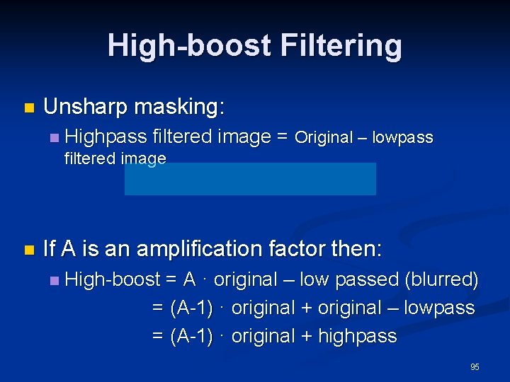
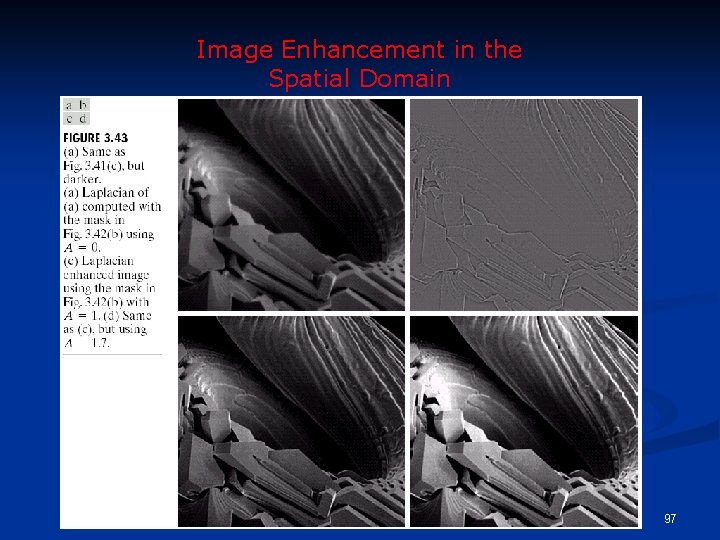
High-boost Filtering n Unsharp masking: n Highpass filtered image = Original – lowpass filtered image n If A is an amplification factor then: n High-boost = A · original – low passed (blurred) = (A-1) · original + original – lowpass = (A-1) · original + highpass 95

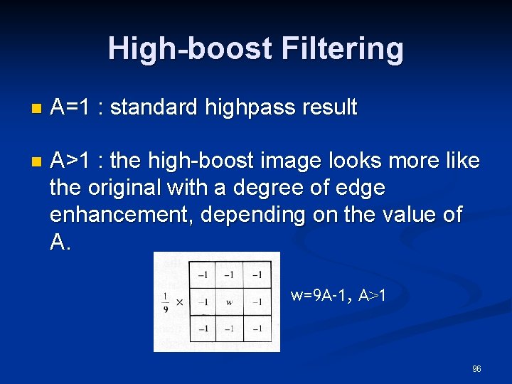
High-boost Filtering n A=1 : standard highpass result n A>1 : the high-boost image looks more like the original with a degree of edge enhancement, depending on the value of A. w=9 A-1, A>1 96

Image Enhancement in the Spatial Domain 97

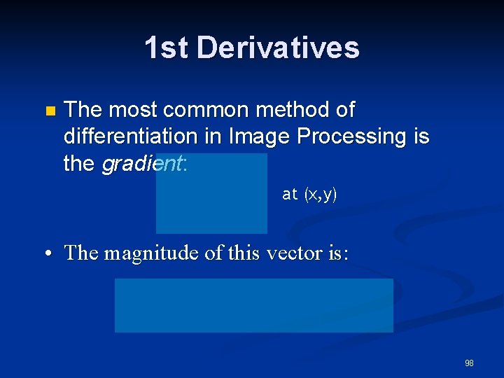
1 st Derivatives n The most common method of differentiation in Image Processing is the gradient: at (x, y) • The magnitude of this vector is: 98

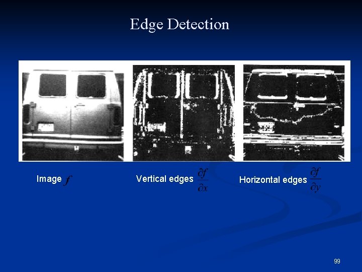
Edge Detection Image Vertical edges Horizontal edges 99

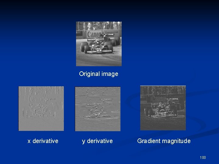
Original image x derivative y derivative Gradient magnitude 100

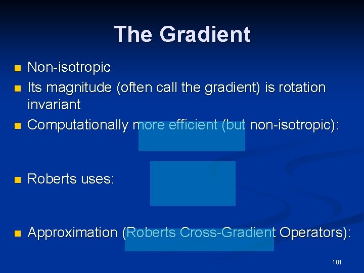
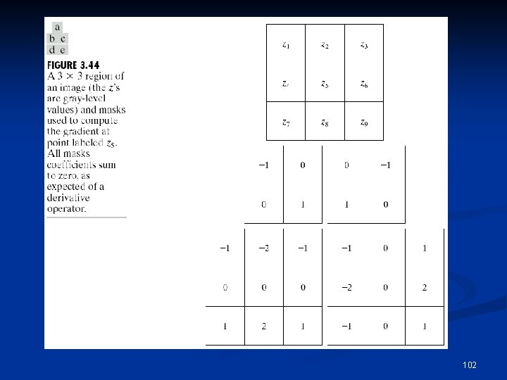
The Gradient n Non-isotropic Its magnitude (often call the gradient) is rotation invariant Computationally more efficient (but non-isotropic): n Roberts uses: n Approximation (Roberts Cross-Gradient Operators): n n 101

102

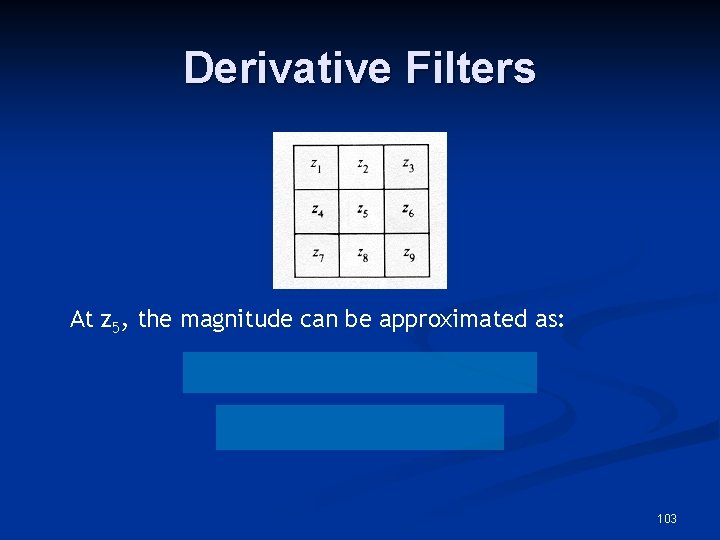
Derivative Filters At z 5, the magnitude can be approximated as: 103

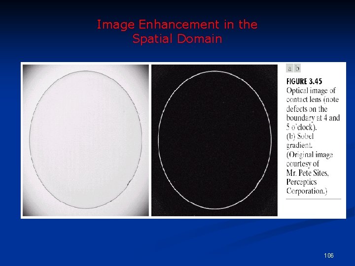
Derivative Filters n Another approach is (Robert): • One last approach is (Sobel Operators): 104

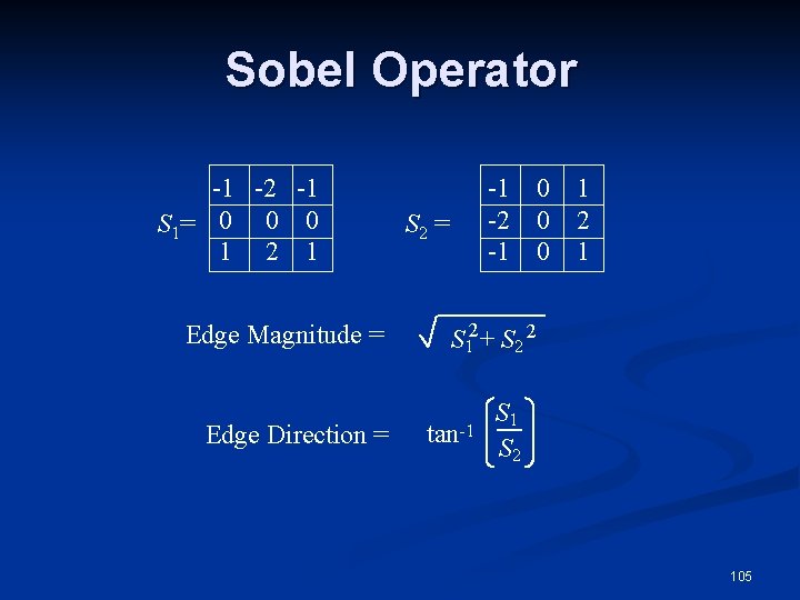
Sobel Operator -1 -2 -1 S 1= 0 0 0 1 2 1 Edge Magnitude = Edge Direction = -1 -2 -1 S 2 = 0 1 0 2 0 1 S 12 + S 2 2 tan-1 S 2 105

Image Enhancement in the Spatial Domain 106

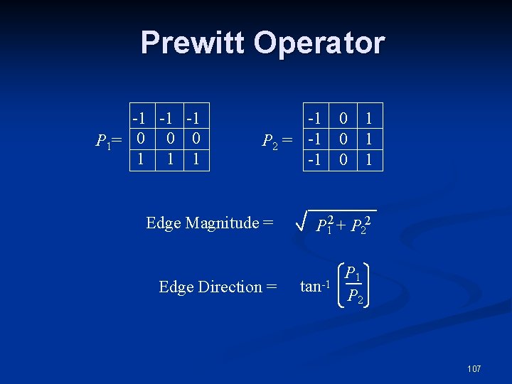
Prewitt Operator -1 -1 -1 P 1= 0 0 0 1 1 1 -1 P 2 = -1 -1 Edge Magnitude = Edge Direction = 0 0 0 1 1 1 P 12 + P 22 tan-1 P 2 107

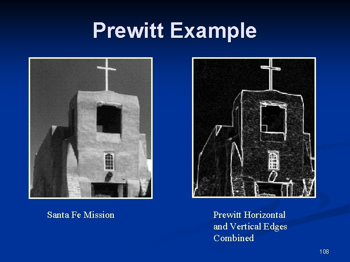
Prewitt Example Santa Fe Mission Prewitt Horizontal and Vertical Edges Combined 108

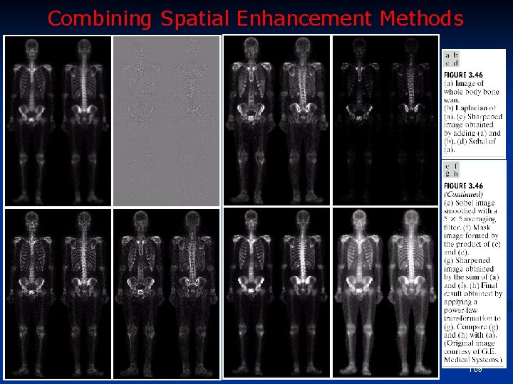
Combining Spatial Enhancement Methods 109