Digital Image Processing Filtering in the Frequency Domain

Digital Image Processing Filtering in the Frequency Domain (Circulant Matrices and Convolution) Christophoros Nikou cnikou@cs. uoi. gr University of Ioannina - Department of Computer Science

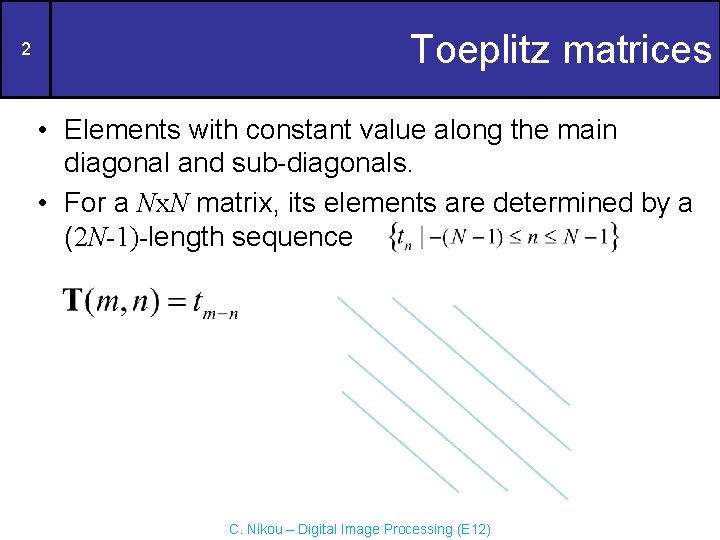
2 Toeplitz matrices • Elements with constant value along the main diagonal and sub-diagonals. • For a Nx. N matrix, its elements are determined by a (2 N-1)-length sequence C. Nikou – Digital Image Processing (E 12)

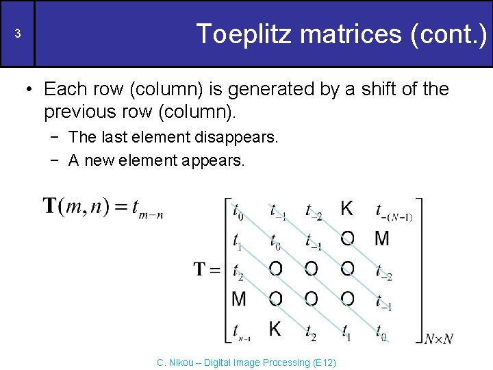
3 Toeplitz matrices (cont. ) • Each row (column) is generated by a shift of the previous row (column). − The last element disappears. − A new element appears. C. Nikou – Digital Image Processing (E 12)

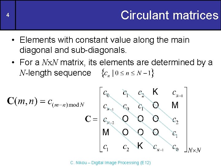
4 Circulant matrices • Elements with constant value along the main diagonal and sub-diagonals. • For a Nx. N matrix, its elements are determined by a N-length sequence C. Nikou – Digital Image Processing (E 12)

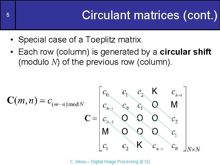
5 Circulant matrices (cont. ) • Special case of a Toeplitz matrix. • Each row (column) is generated by a circular shift (modulo N) of the previous row (column). C. Nikou – Digital Image Processing (E 12)

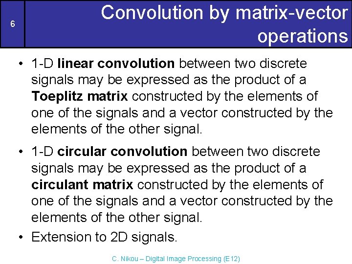
6 Convolution by matrix-vector operations • 1 -D linear convolution between two discrete signals may be expressed as the product of a Toeplitz matrix constructed by the elements of one of the signals and a vector constructed by the elements of the other signal. • 1 -D circular convolution between two discrete signals may be expressed as the product of a circulant matrix constructed by the elements of one of the signals and a vector constructed by the elements of the other signal. • Extension to 2 D signals. C. Nikou – Digital Image Processing (E 12)

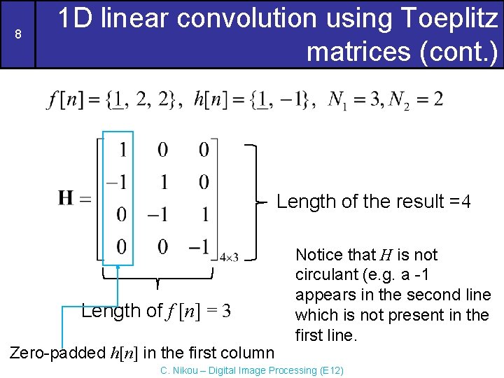
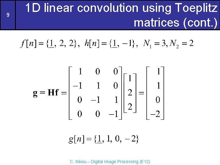
7 1 D linear convolution using Toeplitz matrices • The linear convolution g[n]=f [n]*h [n] will be of length N=N 1+N 2 -1=3+2 -1=4. • We create a Toeplitz matrix H from the elements of h [n] (zero-padded if needed) with − N=4 lines (the length of the result). − N 1=3 columns (the length of f [n]). − The two signals may be interchanged. C. Nikou – Digital Image Processing (E 12)

8 1 D linear convolution using Toeplitz matrices (cont. ) Length of the result =4 Length of f [n] = 3 Zero-padded h[n] in the first column Notice that H is not circulant (e. g. a -1 appears in the second line which is not present in the first line. C. Nikou – Digital Image Processing (E 12)

9 1 D linear convolution using Toeplitz matrices (cont. ) C. Nikou – Digital Image Processing (E 12)

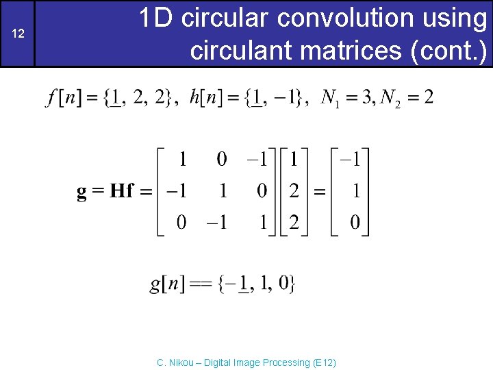
10 1 D circular convolution using circulant matrices • The circular convolution g[n]=f [n] h [n] will be of length N=max{N 1, N 2}=3. • We create a circulant matrix H from the elements of h [n] (zero-padded if needed) of size Nx. N. − The two signals may be interchanged. C. Nikou – Digital Image Processing (E 12)

11 1 D circular convolution using circulant matrices (cont. ) Zero-padded h[n] in the first column C. Nikou – Digital Image Processing (E 12)

12 1 D circular convolution using circulant matrices (cont. ) C. Nikou – Digital Image Processing (E 12)

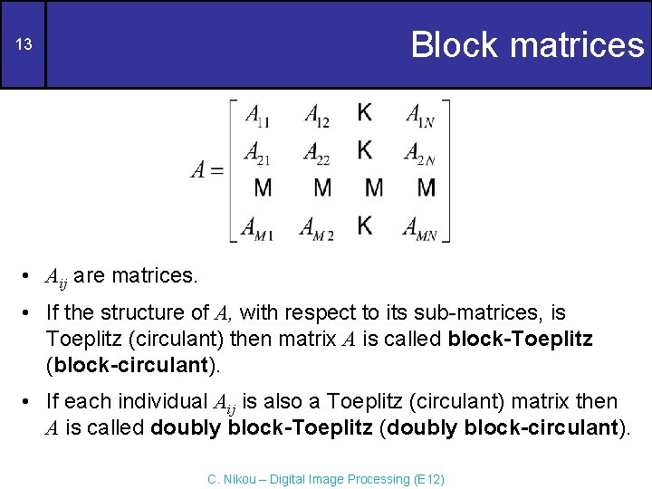
13 Block matrices • Aij are matrices. • If the structure of A, with respect to its sub-matrices, is Toeplitz (circulant) then matrix A is called block-Toeplitz (block-circulant). • If each individual Aij is also a Toeplitz (circulant) matrix then A is called doubly block-Toeplitz (doubly block-circulant). C. Nikou – Digital Image Processing (E 12)

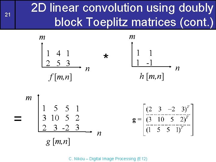
14 2 D linear convolution using doubly block Toeplitz matrices m m 1 4 1 2 5 3 f [m, n] M 1=2, N 1=3 n 1 1 1 -1 h [m, n] n M 2=2, N 2=2 The result will be of size (M 1+M 2 -1) x (N 1+N 2 -1) = 3 x 4 C. Nikou – Digital Image Processing (E 12)

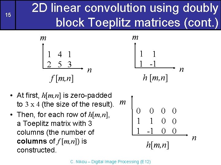
15 2 D linear convolution using doubly block Toeplitz matrices (cont. ) m m 1 4 1 2 5 3 f [m, n] n • At first, h[m, n] is zero-padded to 3 x 4 (the size of the result). m • Then, for each row of h[m, n], a Toeplitz matrix with 3 columns (the number of columns of f [m, n]) is constructed. 1 1 1 -1 h [m, n] 0 0 1 1 0 0 1 -1 0 0 h[m, n] C. Nikou – Digital Image Processing (E 12) n n

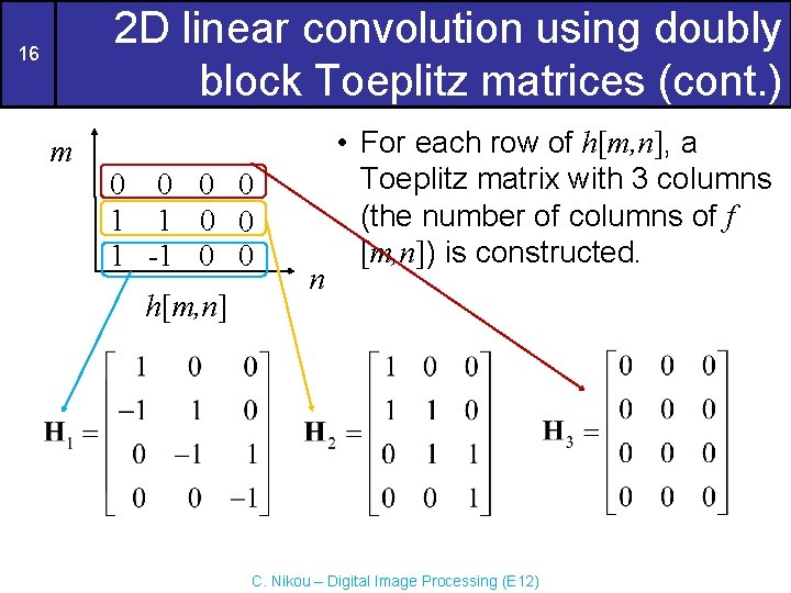
2 D linear convolution using doubly block Toeplitz matrices (cont. ) 16 m 0 0 1 1 0 0 1 -1 0 0 h[m, n] n • For each row of h[m, n], a Toeplitz matrix with 3 columns (the number of columns of f [m, n]) is constructed. C. Nikou – Digital Image Processing (E 12)

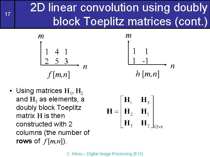
17 2 D linear convolution using doubly block Toeplitz matrices (cont. ) m m 1 4 1 2 5 3 f [m, n] n 1 1 1 -1 h [m, n] • Using matrices H 1, H 2 and H 3 as elements, a doubly block Toeplitz matrix H is then constructed with 2 columns (the number of rows of f [m, n]). C. Nikou – Digital Image Processing (E 12) n

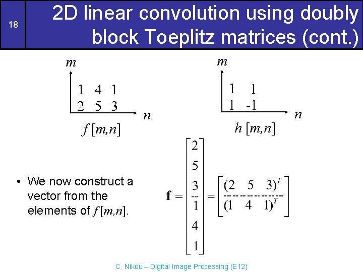
18 2 D linear convolution using doubly block Toeplitz matrices (cont. ) m m 1 4 1 2 5 3 f [m, n] n 1 1 1 -1 h [m, n] • We now construct a vector from the elements of f [m, n]. C. Nikou – Digital Image Processing (E 12) n

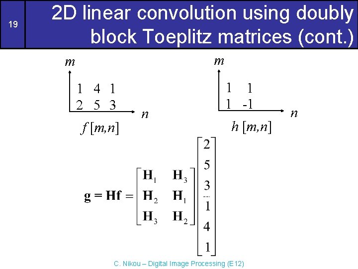
19 2 D linear convolution using doubly block Toeplitz matrices (cont. ) m m 1 4 1 2 5 3 f [m, n] n 1 1 1 -1 h [m, n] C. Nikou – Digital Image Processing (E 12) n

20 2 D linear convolution using doubly block Toeplitz matrices (cont. ) C. Nikou – Digital Image Processing (E 12)

2 D linear convolution using doubly block Toeplitz matrices (cont. ) 21 m m 1 4 1 2 5 3 f [m, n] * n 1 1 1 -1 h [m, n] m = 1 5 5 1 3 10 5 2 2 3 -2 3 g [m, n] n C. Nikou – Digital Image Processing (E 12) n

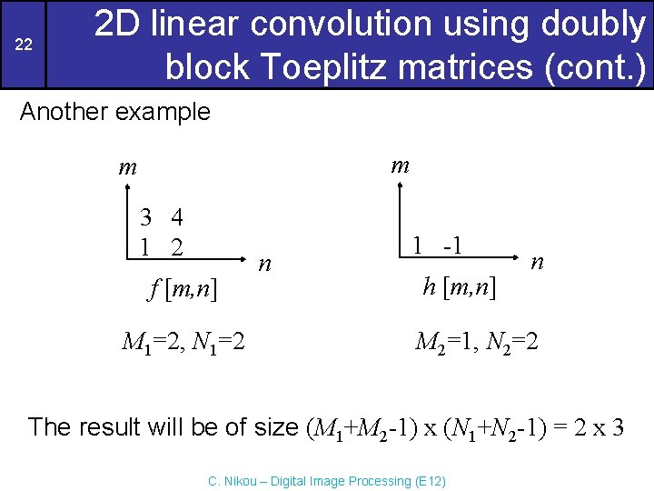
22 2 D linear convolution using doubly block Toeplitz matrices (cont. ) Another example m m 3 4 1 2 f [m, n] M 1=2, N 1=2 n 1 -1 h [m, n] n M 2=1, N 2=2 The result will be of size (M 1+M 2 -1) x (N 1+N 2 -1) = 2 x 3 C. Nikou – Digital Image Processing (E 12)

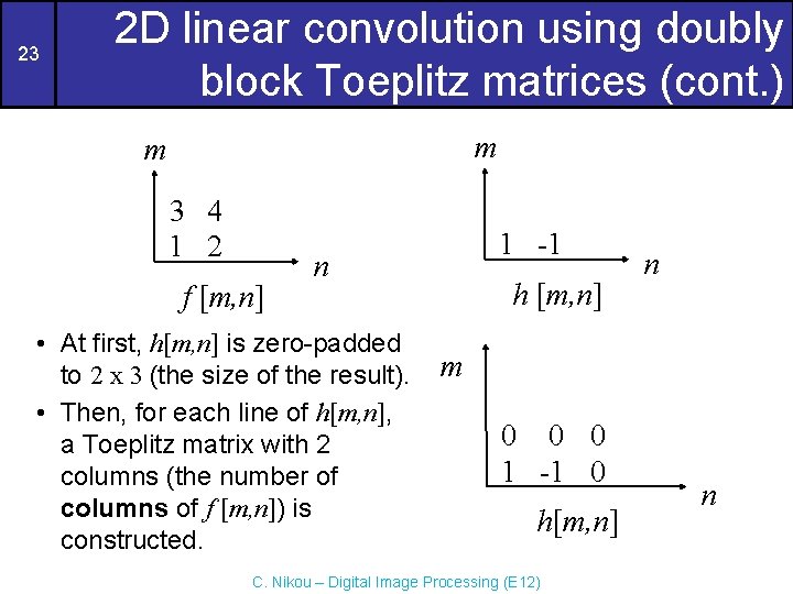
23 2 D linear convolution using doubly block Toeplitz matrices (cont. ) m m 3 4 1 2 f [m, n] 1 -1 n • At first, h[m, n] is zero-padded to 2 x 3 (the size of the result). • Then, for each line of h[m, n], a Toeplitz matrix with 2 columns (the number of columns of f [m, n]) is constructed. h [m, n] n m 0 0 0 1 -1 0 h[m, n] C. Nikou – Digital Image Processing (E 12) n

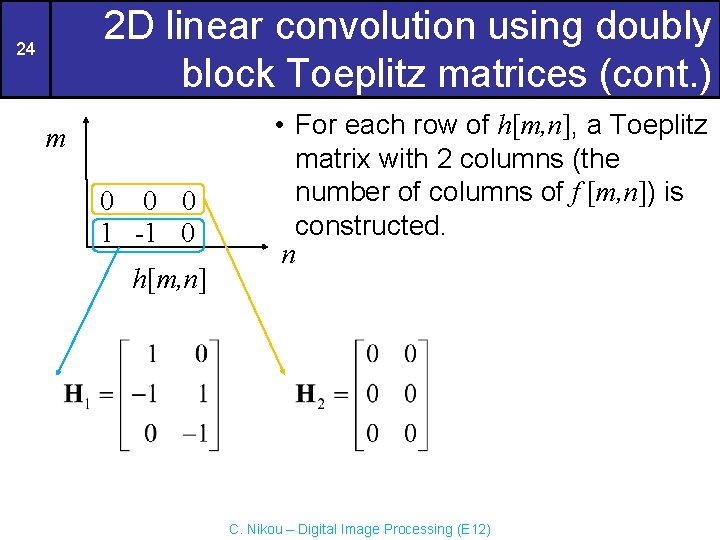
2 D linear convolution using doubly block Toeplitz matrices (cont. ) 24 m 0 0 0 1 -1 0 h[m, n] • For each row of h[m, n], a Toeplitz matrix with 2 columns (the number of columns of f [m, n]) is constructed. n C. Nikou – Digital Image Processing (E 12)

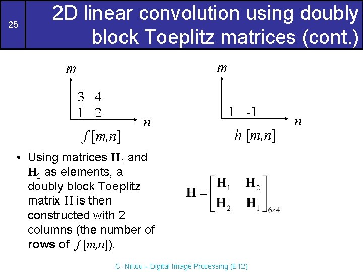
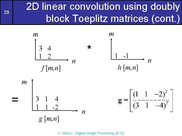
25 2 D linear convolution using doubly block Toeplitz matrices (cont. ) m m 3 4 1 2 f [m, n] n 1 -1 h [m, n] • Using matrices H 1 and H 2 as elements, a doubly block Toeplitz matrix H is then constructed with 2 columns (the number of rows of f [m, n]). C. Nikou – Digital Image Processing (E 12) n

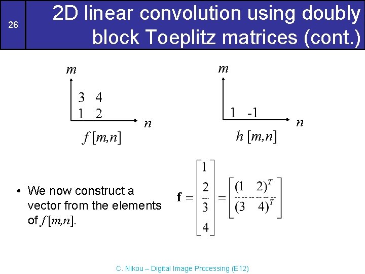
26 2 D linear convolution using doubly block Toeplitz matrices (cont. ) m m 3 4 1 2 f [m, n] n 1 -1 h [m, n] • We now construct a vector from the elements of f [m, n]. C. Nikou – Digital Image Processing (E 12) n

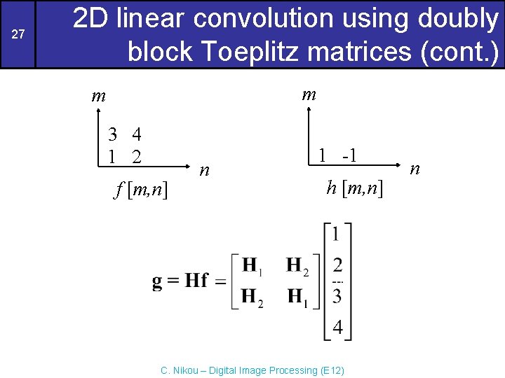
27 2 D linear convolution using doubly block Toeplitz matrices (cont. ) m m 3 4 1 2 f [m, n] n 1 -1 h [m, n] C. Nikou – Digital Image Processing (E 12) n

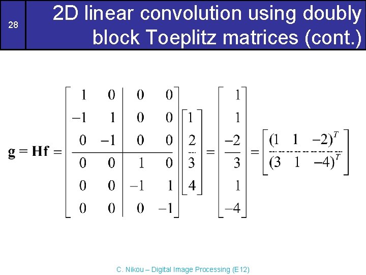
28 2 D linear convolution using doubly block Toeplitz matrices (cont. ) C. Nikou – Digital Image Processing (E 12)

2 D linear convolution using doubly block Toeplitz matrices (cont. ) 29 m m * 3 4 1 2 f [m, n] n 1 -1 h [m, n] m = 3 1 4 1 1 -2 g [m, n] n C. Nikou – Digital Image Processing (E 12) n

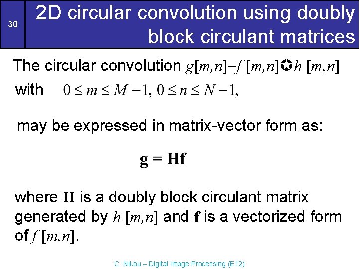
30 2 D circular convolution using doubly block circulant matrices The circular convolution g[m, n]=f [m, n] h [m, n] with may be expressed in matrix-vector form as: where H is a doubly block circulant matrix generated by h [m, n] and f is a vectorized form of f [m, n]. C. Nikou – Digital Image Processing (E 12)

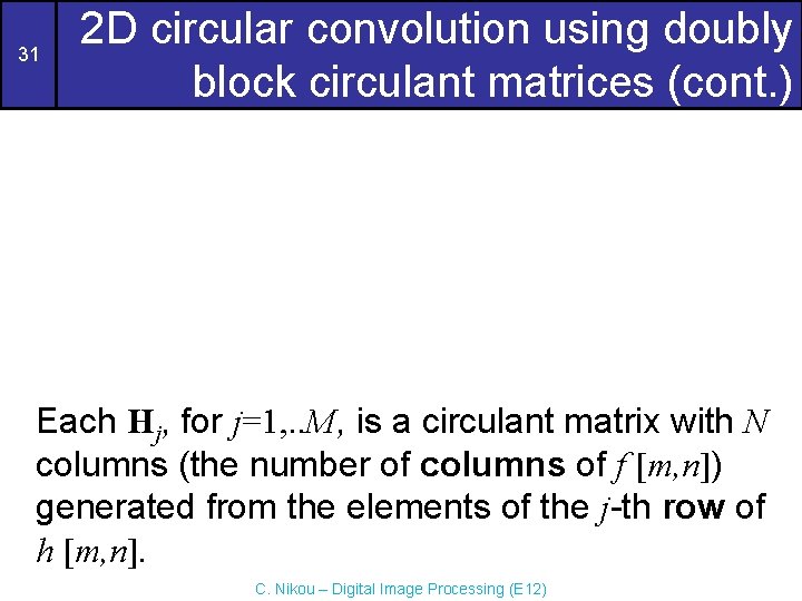
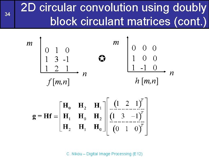
31 2 D circular convolution using doubly block circulant matrices (cont. ) Each Hj, for j=1, . . M, is a circulant matrix with N columns (the number of columns of f [m, n]) generated from the elements of the j-th row of h [m, n]. C. Nikou – Digital Image Processing (E 12)

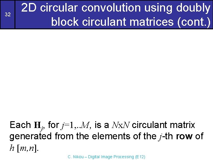
32 2 D circular convolution using doubly block circulant matrices (cont. ) Each Hj, for j=1, . . M, is a Nx. N circulant matrix generated from the elements of the j-th row of h [m, n]. C. Nikou – Digital Image Processing (E 12)

33 2 D circular convolution using doubly block circulant matrices (cont. ) m 0 1 3 -1 1 2 1 f [m, n] m n 0 0 0 1 -1 0 h [m, n] C. Nikou – Digital Image Processing (E 12) n

34 2 D circular convolution using doubly block circulant matrices (cont. ) m 0 1 3 -1 1 2 1 f [m, n] m n 0 0 0 1 -1 0 h [m, n] C. Nikou – Digital Image Processing (E 12) n

35 2 D circular convolution using doubly block circulant matrices (cont. ) C. Nikou – Digital Image Processing (E 12)

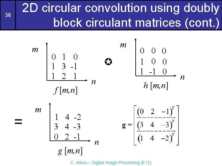
36 2 D circular convolution using doubly block circulant matrices (cont. ) m m 0 1 3 -1 1 2 1 f [m, n] = m 1 4 -2 3 4 -3 0 2 -1 g [m, n] n 0 0 0 1 -1 0 h [m, n] n C. Nikou – Digital Image Processing (E 12) n

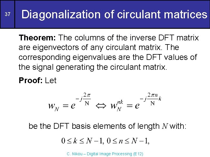
37 Diagonalization of circulant matrices Theorem: The columns of the inverse DFT matrix are eigenvectors of any circulant matrix. The corresponding eigenvalues are the DFT values of the signal generating the circulant matrix. Proof: Let be the DFT basis elements of length N with: C. Nikou – Digital Image Processing (E 12)

38 Diagonalization of circulant matrices (cont. ) We know that the DFT F [k] of a 1 D signal f [n] may be expressed in matrix-vector form: where C. Nikou – Digital Image Processing (E 12)

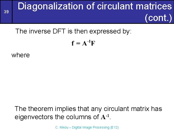
39 Diagonalization of circulant matrices (cont. ) The inverse DFT is then expressed by: where The theorem implies that any circulant matrix has eigenvectors the columns of A-1. C. Nikou – Digital Image Processing (E 12)

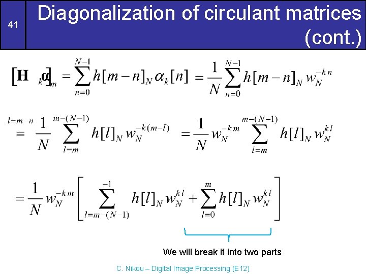
40 Diagonalization of circulant matrices (cont. ) Let H be a Nx. N circulant matrix generated by the 1 D N-length signal h[n], that is: Let also αk be the k-th column of the inverse DFT matrix A-1. We will prove that αk, for any k, is an eigenvector of H. The m-th element of the vector Hαk, denoted by is the result of the circular convolution of the signal h[n] with αk. C. Nikou – Digital Image Processing (E 12)

41 Diagonalization of circulant matrices (cont. ) We will break it into two parts C. Nikou – Digital Image Processing (E 12)

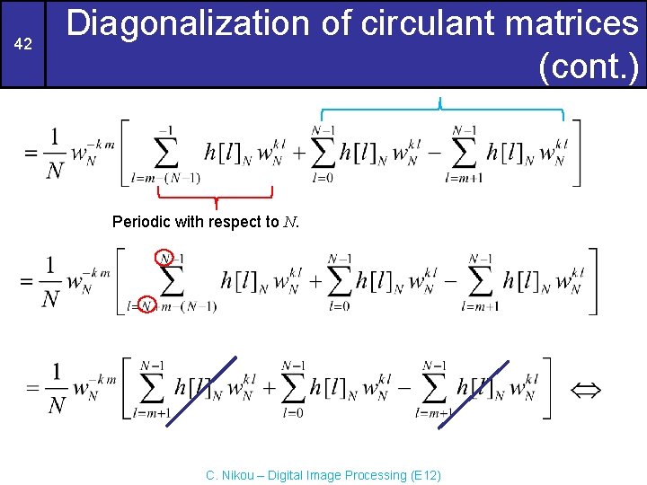
42 Diagonalization of circulant matrices (cont. ) Periodic with respect to N. C. Nikou – Digital Image Processing (E 12)

43 Diagonalization of circulant matrices (cont. ) DFT of h[n] at k. This holds for any value of m. Therefore: which means that αk, for any k, is an eigenvector of H with corresponding eigenvalue the k-th element of H[k], the DFT of the signal generating H. C. Nikou – Digital Image Processing (E 12)

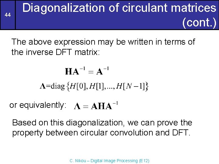
44 Diagonalization of circulant matrices (cont. ) The above expression may be written in terms of the inverse DFT matrix: or equivalently: Based on this diagonalization, we can prove the property between circular convolution and DFT. C. Nikou – Digital Image Processing (E 12)

45 Diagonalization of circulant matrices (cont. ) DFT of g[n] DFT of h [n] C. Nikou – Digital Image Processing (E 12) DFT of f [n]

46 Diagonalization of doubly block circulant matrices • These properties may be generalized in 2 D. • We need to define the Kronecker product: C. Nikou – Digital Image Processing (E 12)

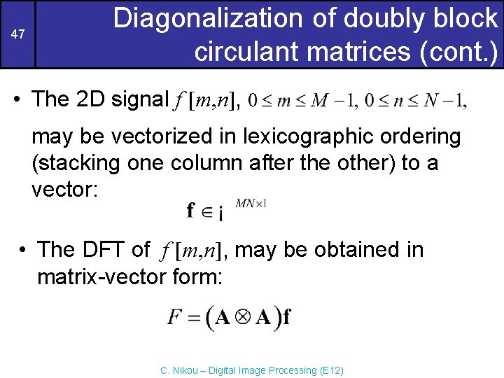
47 Diagonalization of doubly block circulant matrices (cont. ) • The 2 D signal f [m, n], may be vectorized in lexicographic ordering (stacking one column after the other) to a vector: • The DFT of f [m, n], may be obtained in matrix-vector form: C. Nikou – Digital Image Processing (E 12)

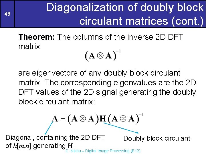
48 Diagonalization of doubly block circulant matrices (cont. ) Theorem: The columns of the inverse 2 D DFT matrix are eigenvectors of any doubly block circulant matrix. The corresponding eigenvalues are the 2 D DFT values of the 2 D signal generating the doubly block circulant matrix: Diagonal, containing the 2 D DFT of h[m, n] generating H Doubly block circulant C. Nikou – Digital Image Processing (E 12)