Digital Image Processing Classification Samples in the feature

Digital Image Processing Classification

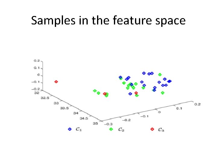
Samples in the feature space

Supervised Classification • Non-parametric – K-Nearest Neighbours • Parametric – Support Vector Machines – Random Forests – Neural Networks – Convolution Neural Networks

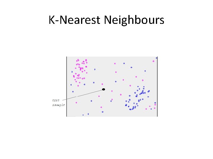
K-Nearest Neighbours • Given a set of pre-classified (seen) data instances, it is required to search for the most similar ones to the test (unseen) sample within these instances. • A test sample is classified by a majority vote of its neighbors, with the object being assigned to the class most common among its k nearest neighbors (k is a positive integer, typically small). If k = 1, then the object is simply assigned to the class of that single nearest neighbor. • The most intuitive to humans • Computationally intensive • Low accuracy in noisy data

K-Nearest Neighbours

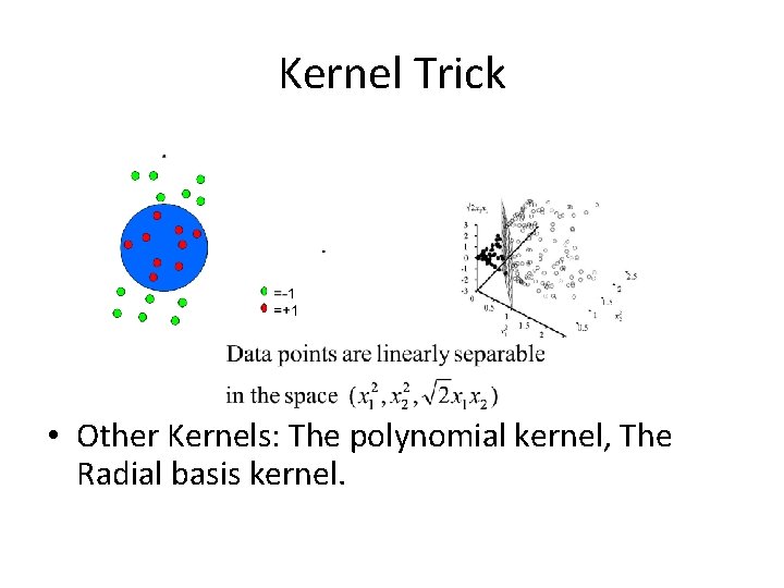
Support Vector Machine (SVM) • Max-Margin Classifier – Formalize notion of the best linear separator • Lagrangian Multipliers – Way to convert a constrained optimization problem to one that is easier to solve • Kernels – Projecting data into higher-dimensional space makes it linearly separable • Adapted to n- classes

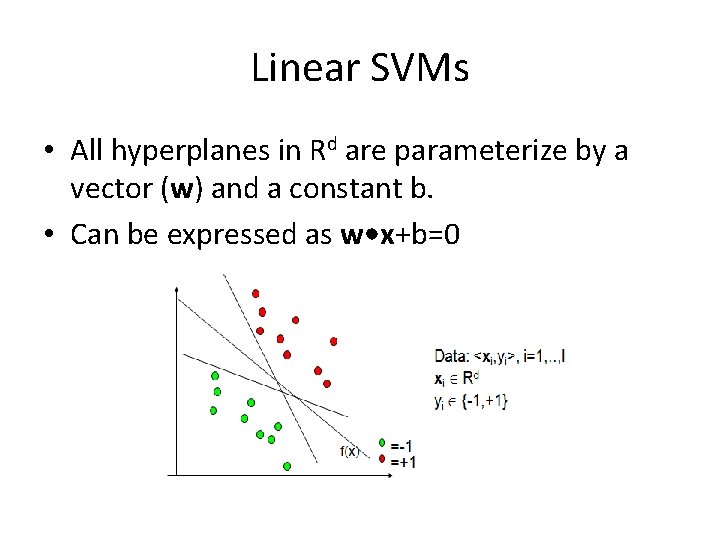
Linear SVMs • All hyperplanes in Rd are parameterize by a vector (w) and a constant b. • Can be expressed as w • x+b=0

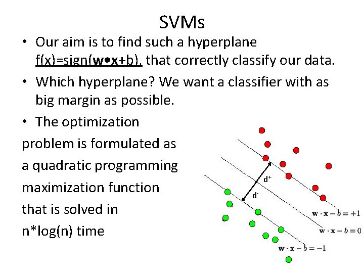
SVMs • Our aim is to find such a hyperplane f(x)=sign(w • x+b), that correctly classify our data. • Which hyperplane? We want a classifier with as big margin as possible. • The optimization problem is formulated as a quadratic programming d maximization function d that is solved in n*log(n) time + -

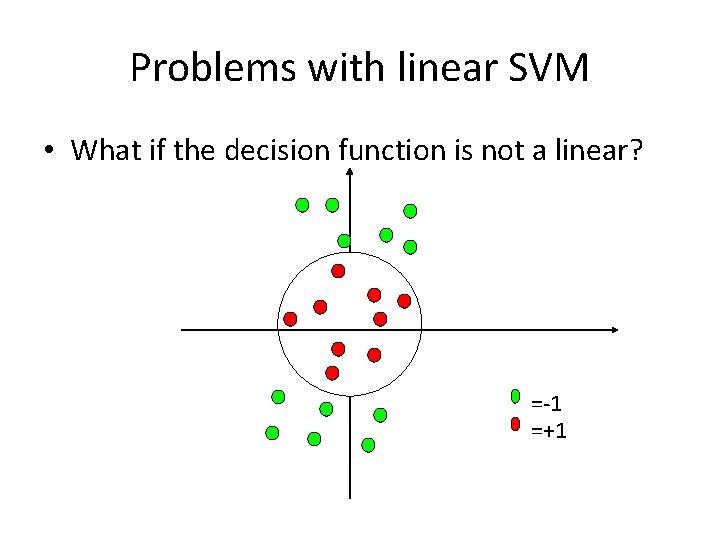
Problems with linear SVM • What if the decision function is not a linear? =-1 =+1

Kernel Trick • Other Kernels: The polynomial kernel, The Radial basis kernel.

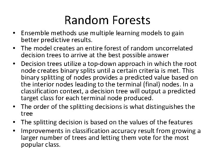
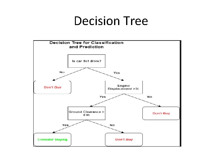
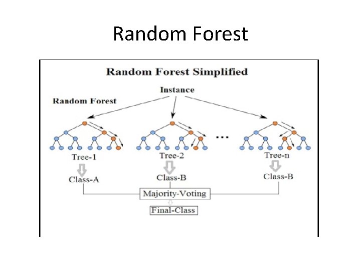
Random Forests • Ensemble methods use multiple learning models to gain better predictive results. • The model creates an entire forest of random uncorrelated decision trees to arrive at the best possible answer • Decision trees utilize a top-down approach in which the root node creates binary splits until a certain criteria is met. This binary splitting of nodes provides a predicted value based on the interior nodes leading to the terminal (final) nodes. In a classification context, a decision tree will output a predicted target class for each terminal node produced. • The order of the splitting decisions is what distinguishes the tree • The splitting decision is based on the values of the features • Improvements in classification accuracy result from growing a larger number of trees and letting them vote for the most popular class.

Decision Tree

Random Forest

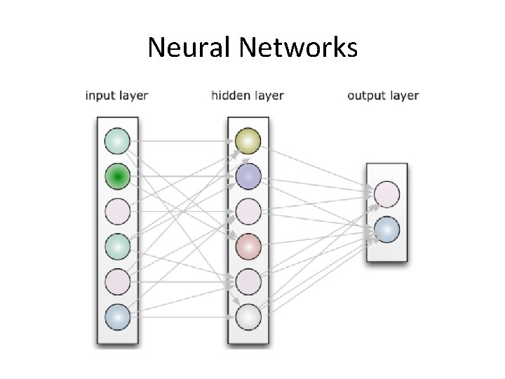
Neural Networks

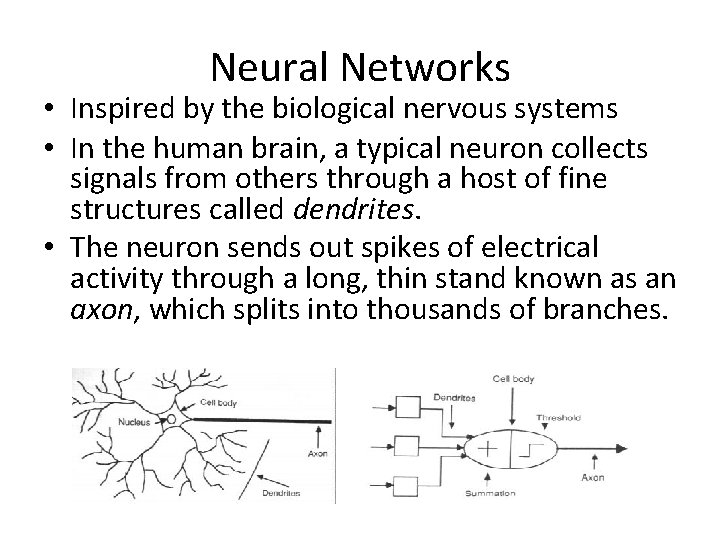
Neural Networks • Inspired by the biological nervous systems • In the human brain, a typical neuron collects signals from others through a host of fine structures called dendrites. • The neuron sends out spikes of electrical activity through a long, thin stand known as an axon, which splits into thousands of branches.

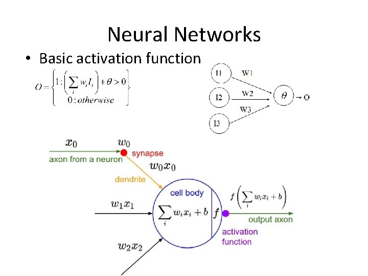
Neural Networks • Basic activation function

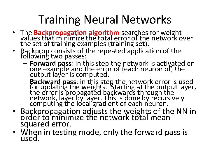
Training Neural Networks • The Backpropagation algorithm searches for weight values that minimize the total error of the network over the set of training examples (training set). • Backprop consists of the repeated application of the following two passes: – Forward pass: in this step the network is activated on one example and the error of (each neuron of) the output layer is computed. – Backward pass: in this step the network error is used for updating the weights. Starting at the output layer, the error is propagated backwards through the network, layer by layer. This is done by recursively computing the local gradient of each neuron. • Backpropagation adjusts the weights of the NN in order to minimize the network total mean squared error. • When in testing mode, only the forward pass is used.

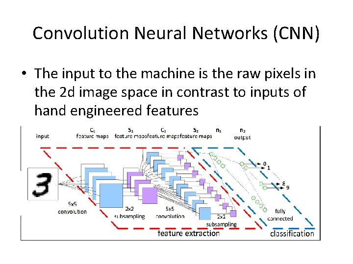
Convolution Neural Networks (CNN) • The input to the machine is the raw pixels in the 2 d image space in contrast to inputs of hand engineered features

Comment on classification accuracy • "Generalization" refers to the ability of a classifier to correctly classify instances that it has not yet seen as part of its training and is always a desirable feature. • Generalization error can be minimized by avoiding overfitting in the learning algorithm. • Performance during learning iterations is monitored through training and testing errors • Overfitting refers to a model that models the training data too well. Overfitting happens when a model learns the detail and noise in the training data to the extent that it negatively impacts the performance of the model on new data.