Digital Image Processing Chapter 3 Intensity Transformations and


 l A small 2 -D array in which")


")
 is the desired PDF")
")


 in the neighborhood is the")

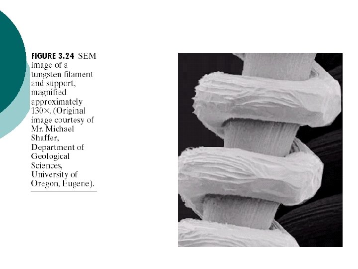
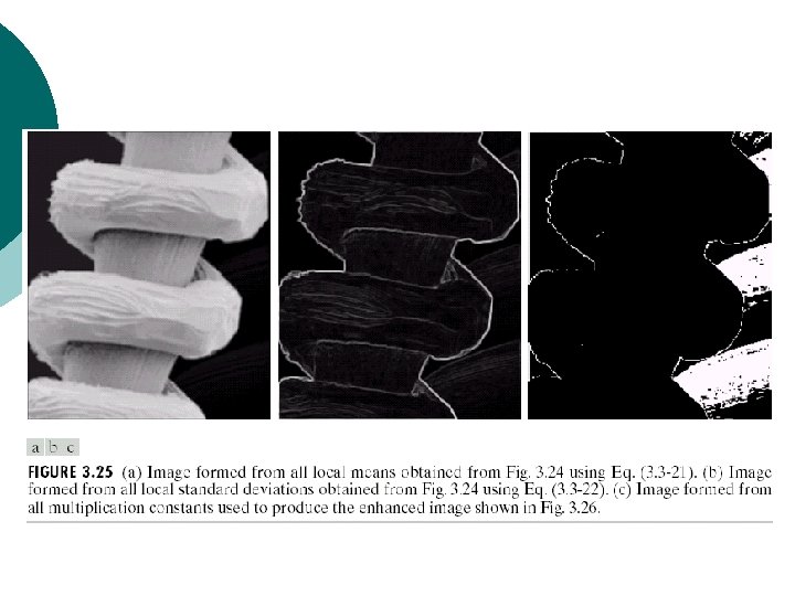


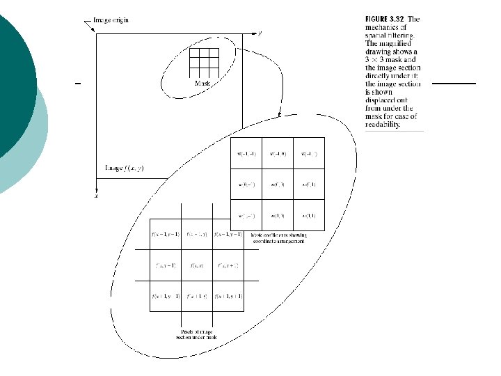
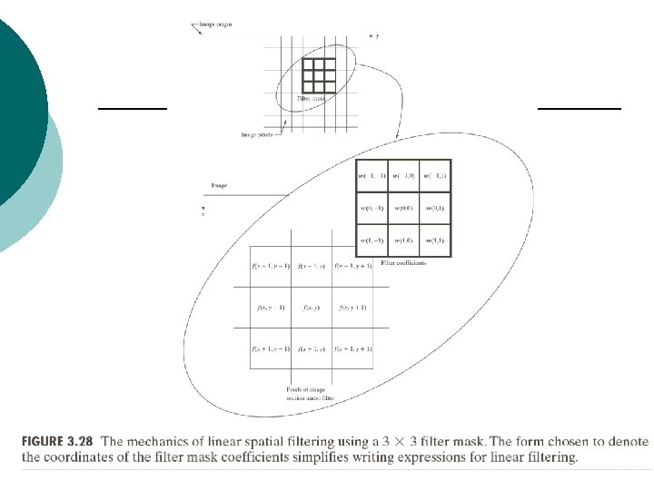

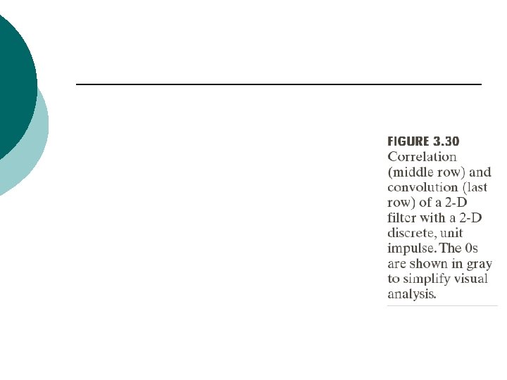


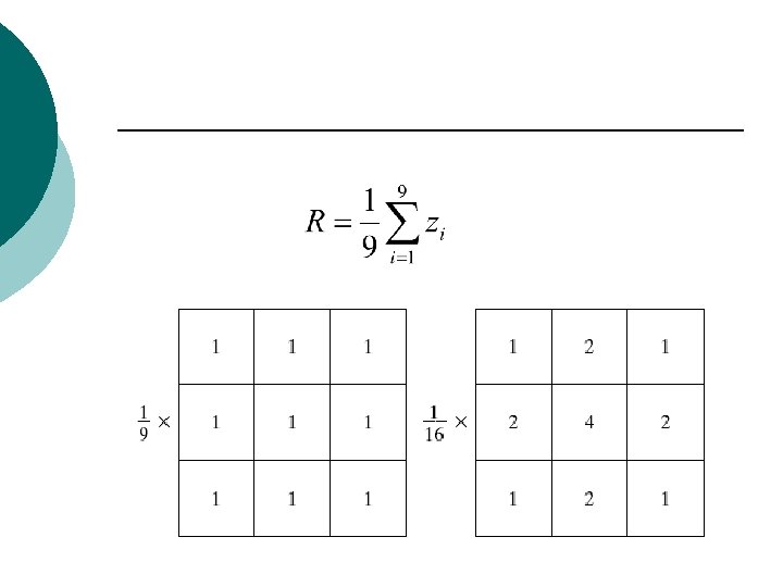
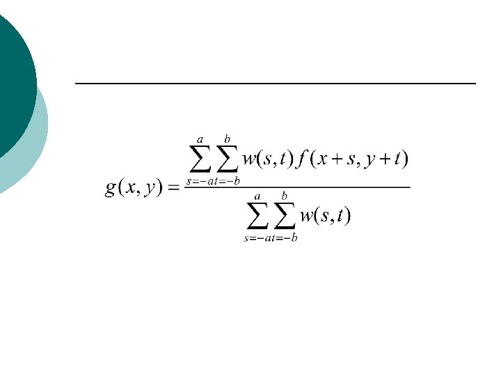
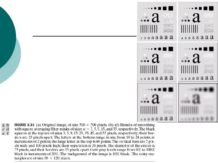
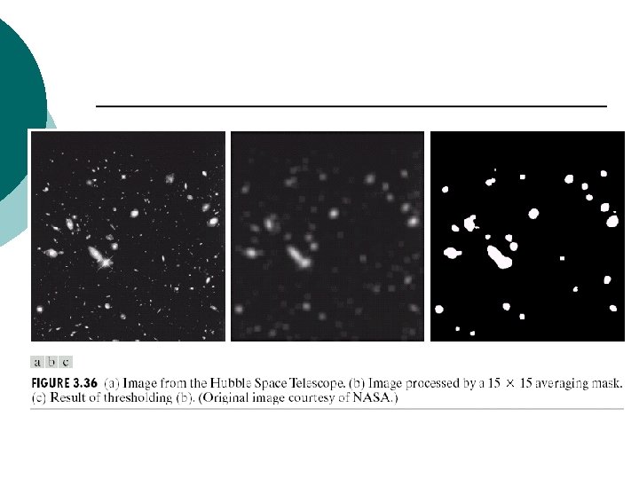

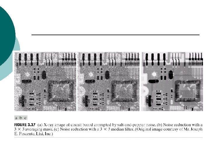

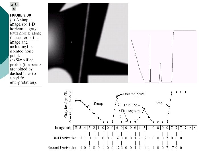
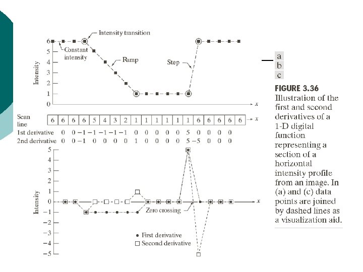

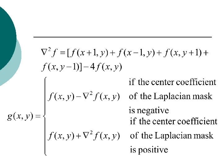
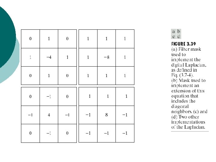
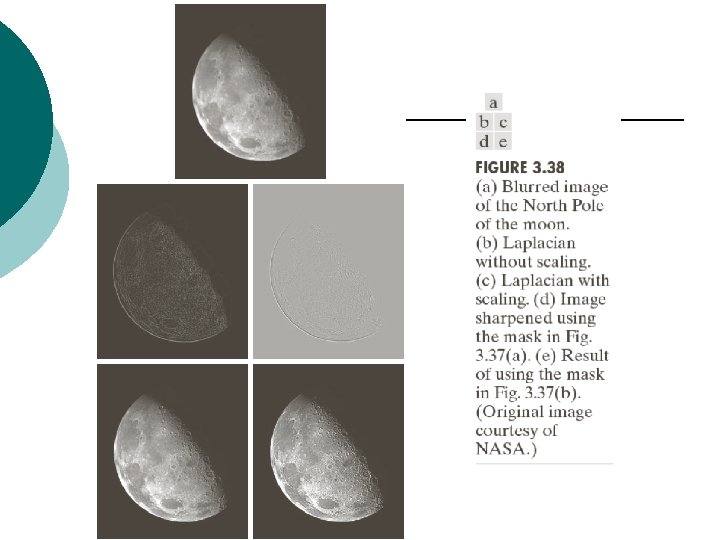

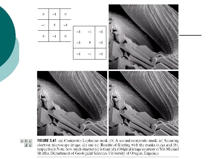


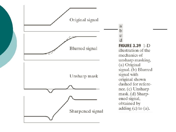
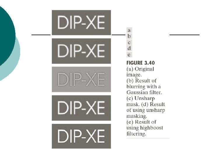
 image sharpening—The gradient")
")


- Slides: 93
Digital Image Processing Chapter 3: Intensity Transformations and Spatial Filtering
Background ¡ Spatial domain process l where is the input image, is the processed image, and T is an operator on f, defined over some neighborhood of
¡ Neighborhood about a point
¡ Gray-level transformation function l where r is the gray level of s is the gray level of point and at any
¡ Contrast enhancement l For example, a thresholding function
¡ Masks (filters, kernels, templates, windows) l A small 2 -D array in which the values of the mask coefficients determine the nature of the process
Some Basic Gray Level Transformations
¡ Image negatives l Enhance white or gray details
¡ Log transformations l Compress the dynamic range of images with large variations in pixel values
l From the range 00 to 6. 2 to the range
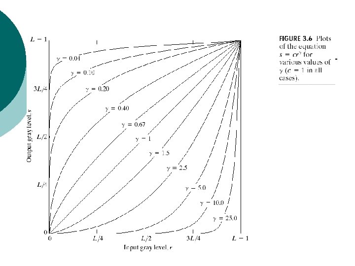
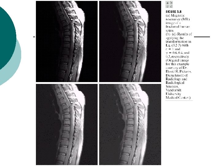
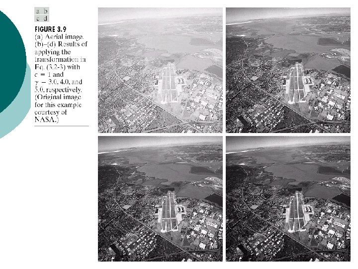
Power-law transformations ¡ or ¡ l l maps a narrow range of dark input values into a wider range of output values, while maps a narrow range of bright input values into a wider range of output values : gamma, gamma correction
¡ Monitor,
¡ Piecewise-linear transformation functions l The form of piecewise functions can be arbitrarily complex
l Contrast stretching
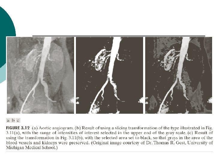
l Gray-level slicing
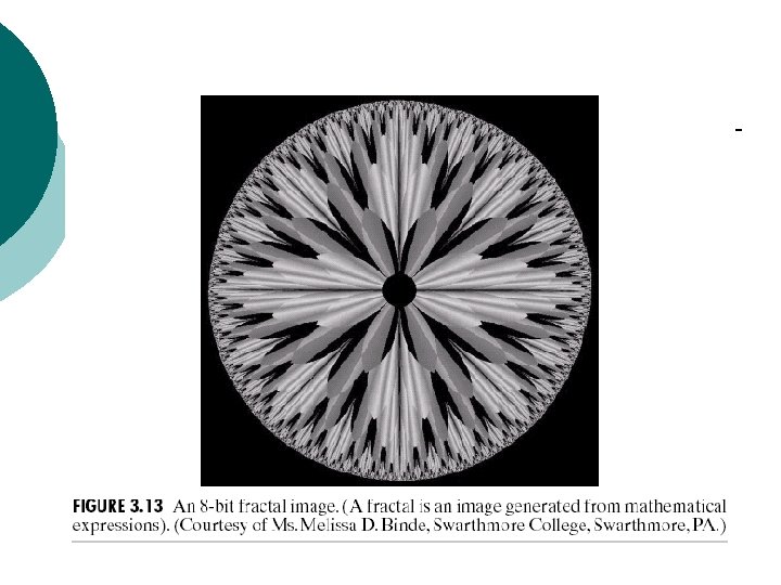
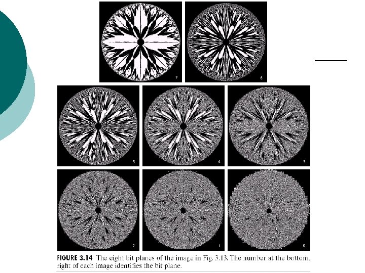
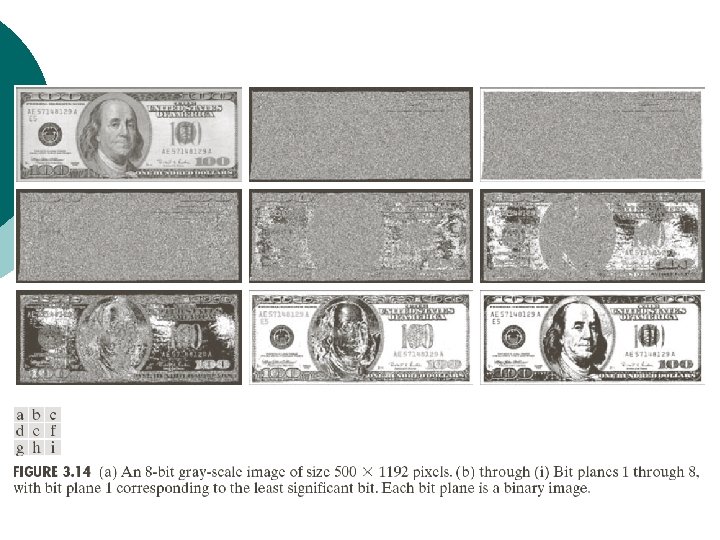
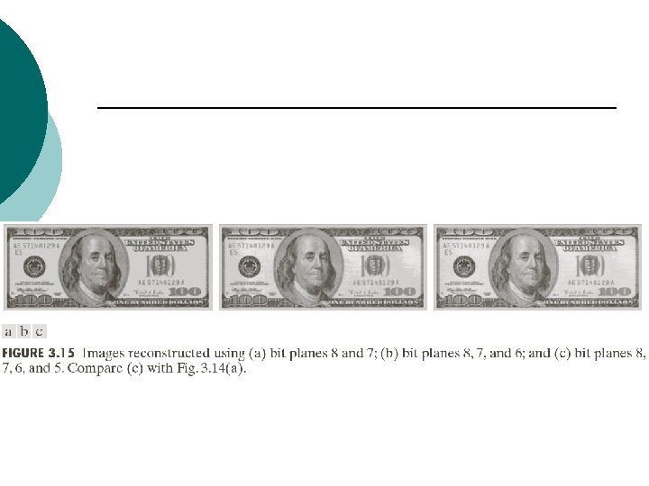
l Bit-plane slicing
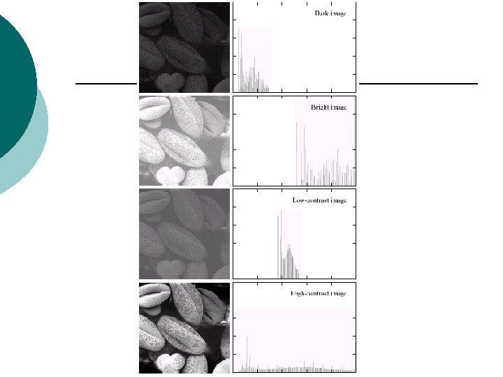
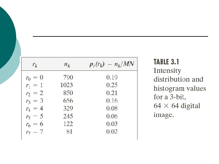
Histogram Processing ¡ Histogram l l where is the kth gray level and the number of pixels in the image having gray level Normalized histogram is
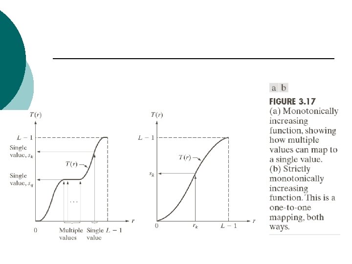
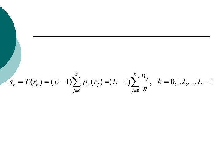
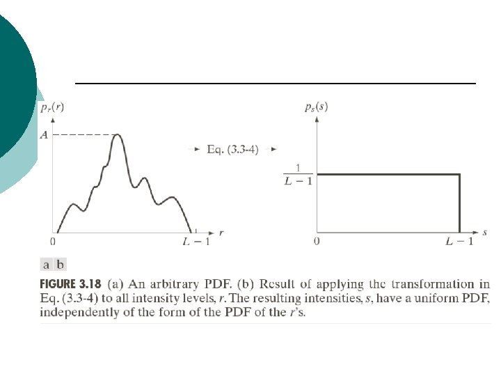
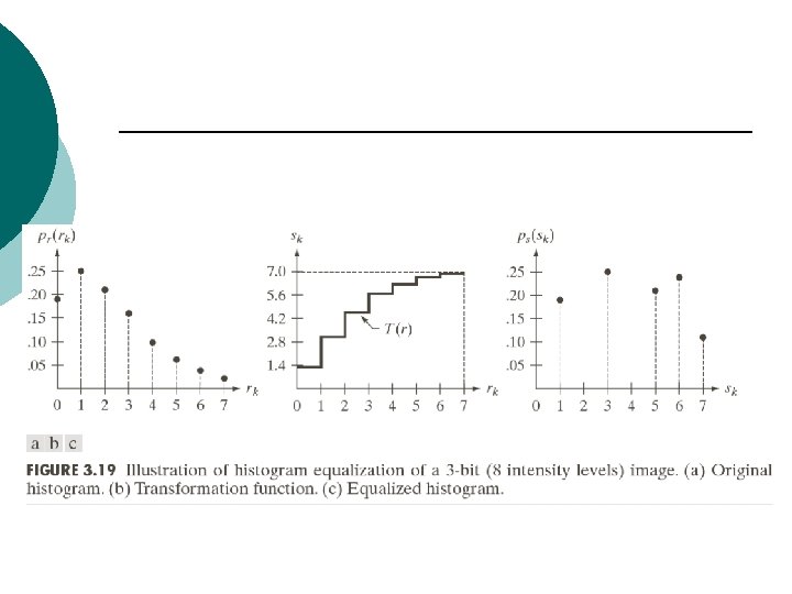
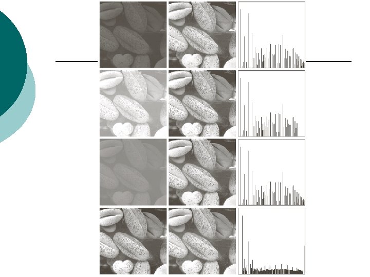
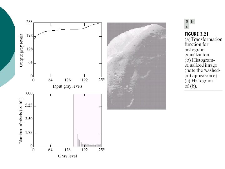
¡ Histogram equalization
l Probability density functions (PDF)
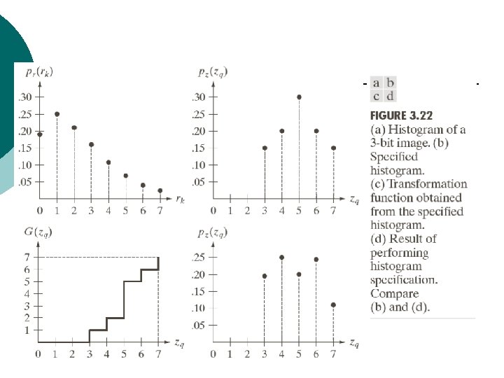
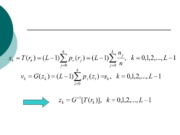
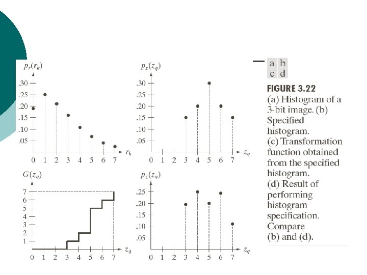
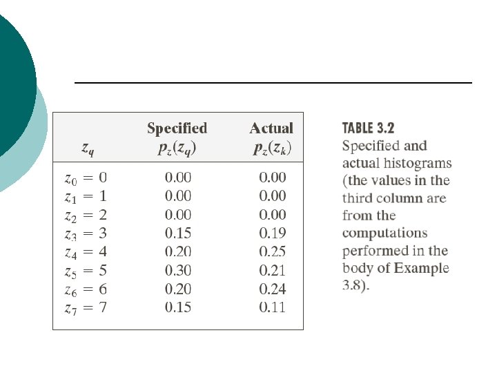
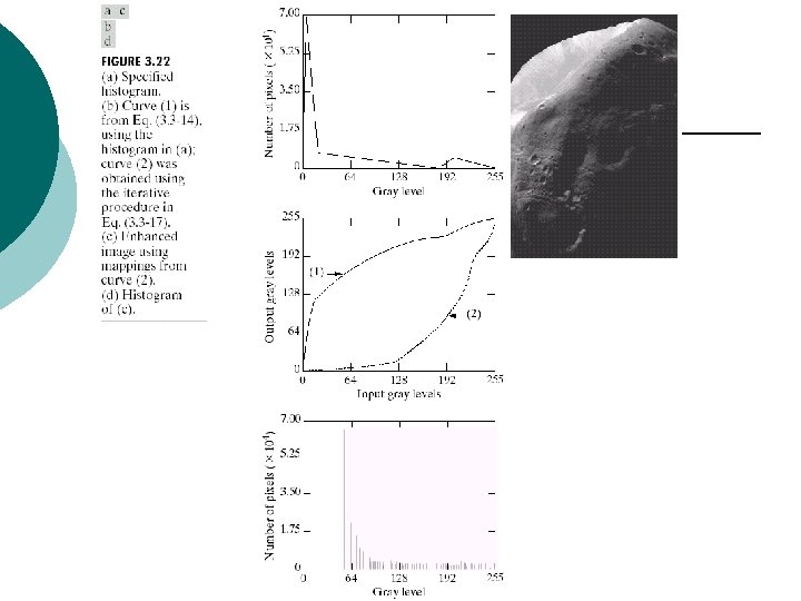
¡ Histogram matching (specification) is the desired PDF
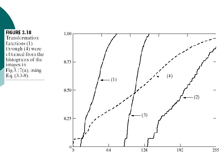
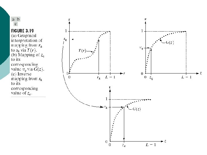
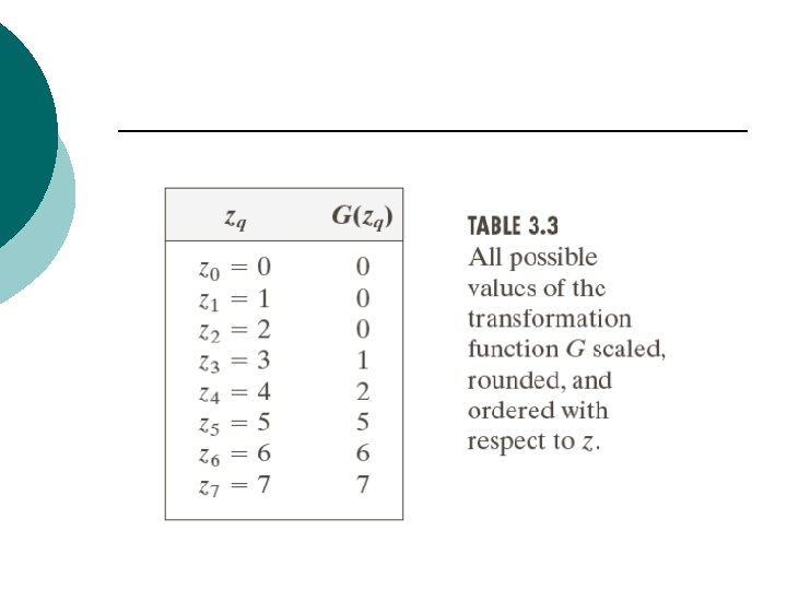
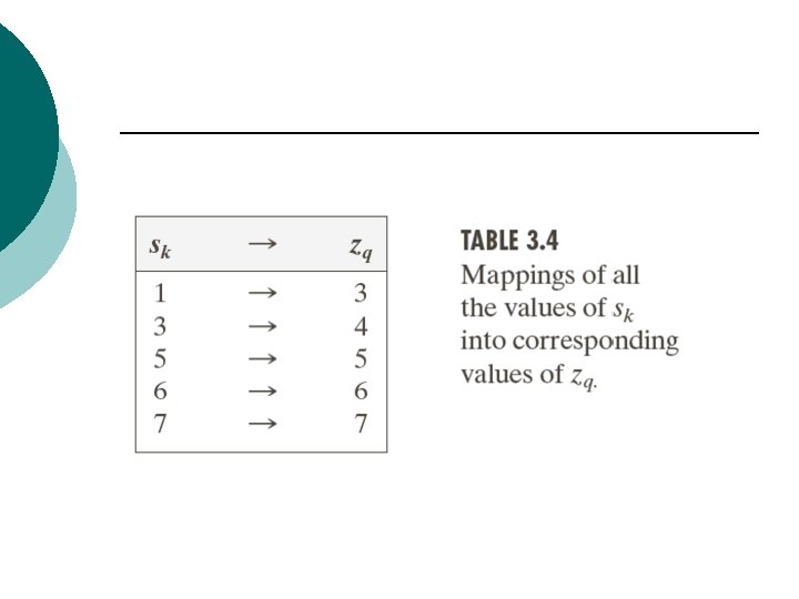
¡ Histogram matching l l l Obtain the histogram of the given image, T(r) Precompute a mapped level for each level Obtain the transformation function G from the given Precompute for each value of Map to its corresponding level ; then map level into the final level
¡ Local enhancement l Histogram using a local neighborhood, for example 7*7 neighborhood
l Histogram using a local 3*3 neighborhood
¡ Use of histogram statistics for image enhancement l l l denotes a discrete random variable denotes the normalized histogram component corresponding to the ith value of Mean
l The nth moment l The second moment
l l Global enhancement: The global mean and variance are measured over an entire image Local enhancement: The local mean and variance are used as the basis for making changes
l is the gray level at coordinates (s, t) in the neighborhood is the neighborhood normalized histogram component mean: l local variance l l
l l are specified parameters is the global mean is the global standard deviation Mapping
Fundamentals of Spatial Filtering ¡ The Mechanics of Spatial Filtering
l l Image size: Mask size: and
¡ Spatial Correlation and Convolution
¡ Vector Representation of Linear Filtering
Smoothing Spatial Filters ¡ Smoothing Linear Filters l l l Noise reduction Smoothing of false contours Reduction of irrelevant detail
¡ Order-statistic filters l l median filter: Replace the value of a pixel by the median of the gray levels in the neighborhood of that pixel Noise-reduction
Sharpening Spatial Filters ¡ Foundation l The first-order derivative l The second-order derivative
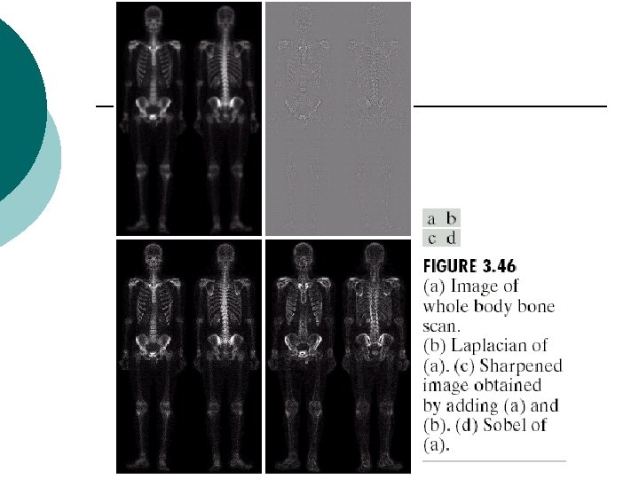
¡ Use of second derivatives for enhancement-The Laplacian l Development of the method
l Simplifications
¡ Unsharp masking and highboost filtering l Unsharp masking ¡ ¡ Substract a blurred version of an image from the image itself : The image, blurred image : The
l High-boost filtering
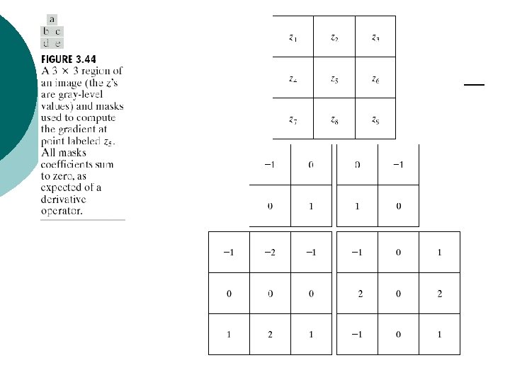
¡ Using first-order derivatives for (nonlinear) image sharpening—The gradient
l The magnitude is rotation invariant (isotropic)
l Computing using cross differences, Roberts cross-gradient operators and
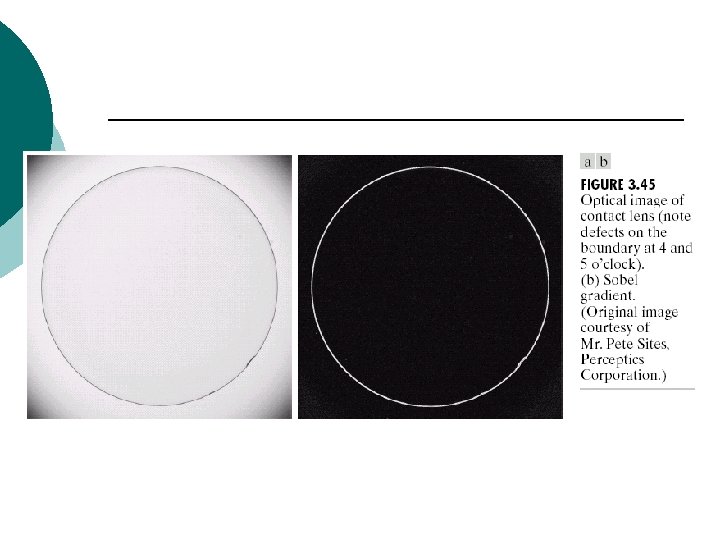
l Sobel operators ¡ A weight value of 2 is to achieve some smoothing by giving more importance to the center point
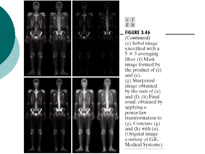
Combining Spatial Enhancement Methods ¡ An example l l Laplacian to highlight fine detail Gradient to enhance prominent edges Smoothed version of the gradient image used to mask the Laplacian image Increase the dynamic range of the gray levels by using a gray-level transformation