Digital Image Processing Chapter 3 Image Enhancement in

Digital Image Processing Chapter 3: Image Enhancement in the Spatial Domain

Background ¡ Spatial domain process l where is the input image, is the processed image, and T is an operator on f, defined over some neighborhood of

¡ Neighborhood about a point

¡ Gray-level transformation function l where r is the gray level of s is the gray level of point and at any

¡ Contrast enhancement l For example, a thresholding function

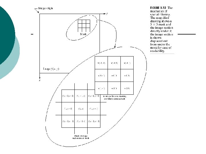
¡ Masks (filters, kernels, templates, windows) l A small 2 -D array in which the values of the mask coefficients determine the nature of the process

Some Basic Gray Level Transformations

¡ Image negatives l Enhance white or gray details

¡ Log transformations l Compress the dynamic range of images with large variations in pixel values

l From the range 00 to 6. 2 to the range

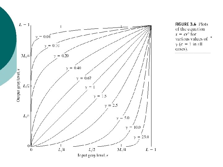
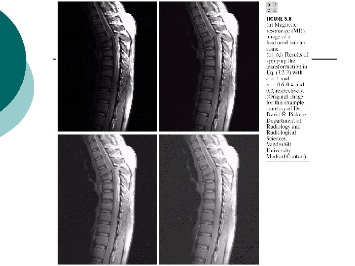
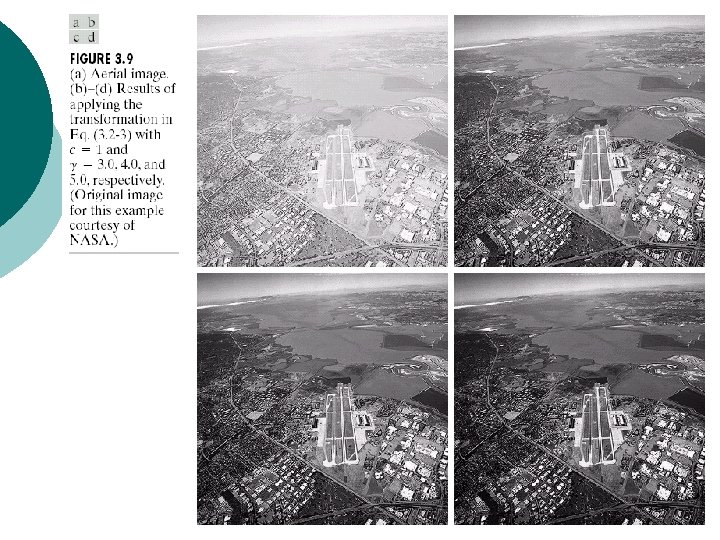
Power-law transformations ¡ or ¡ l l maps a narrow range of dark input values into a wider range of output values, while maps a narrow range of bright input values into a wider range of output values : gamma, gamma correction

¡ Monitor,

¡ Piecewise-linear transformation functions l The form of piecewise functions can be arbitrarily complex

l Contrast stretching

l Gray-level slicing

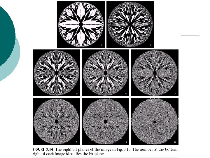
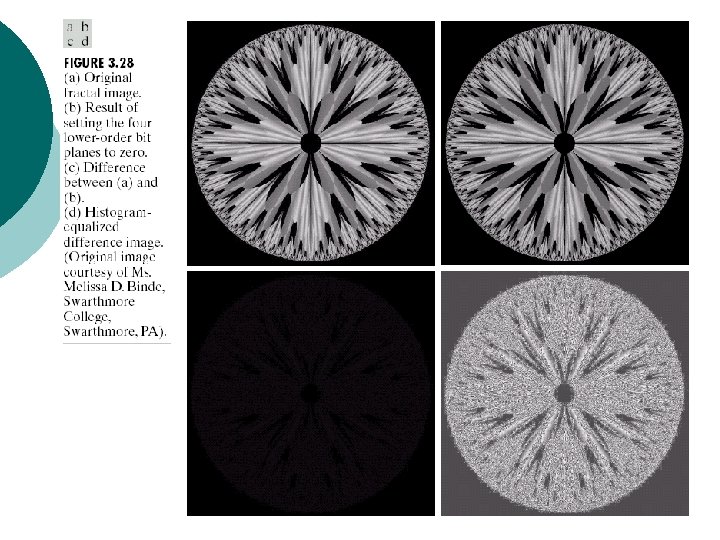
l Bit-plane slicing

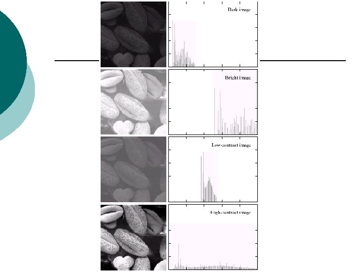
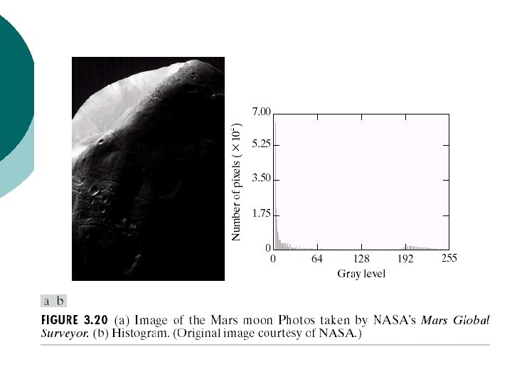
Histogram Processing ¡ Histogram l l where is the kth gray level and the number of pixels in the image having gray level Normalized histogram is

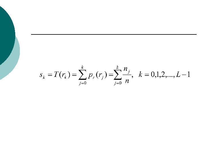
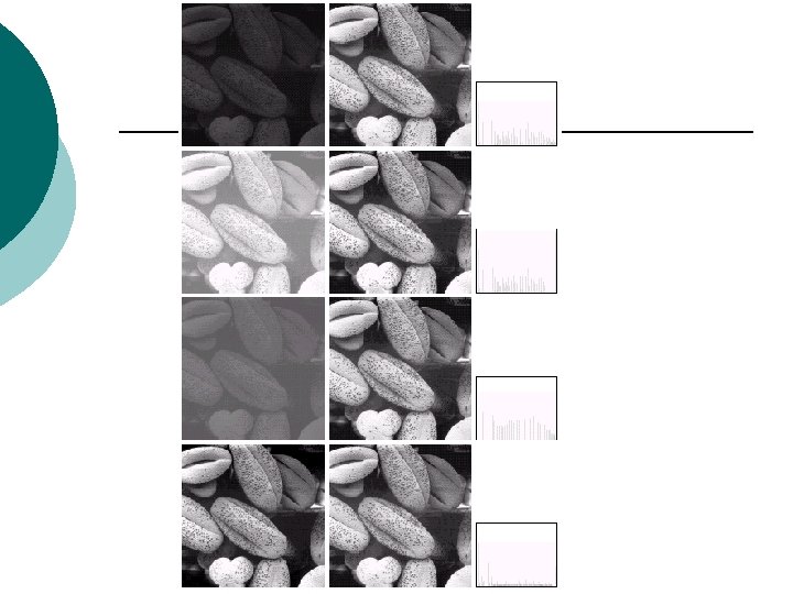
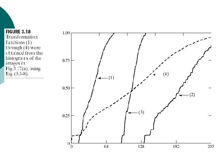
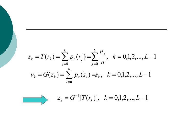
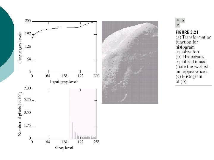
¡ Histogram equalization

l Probability density functions (PDF)

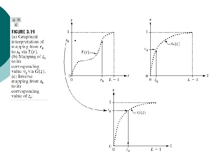
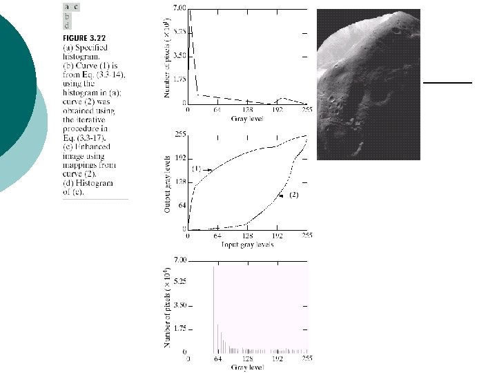
¡ Histogram matching (specification) is the desired PDF

¡ Histogram matching l l l Obtain the histogram of the given image, T(r) Precompute a mapped level for each level Obtain the transformation function G from the given Precompute for each value of Map to its corresponding level ; then map level into the final level

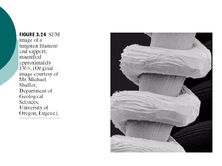
¡ Local enhancement l Histogram using a local neighborhood, for example 7*7 neighborhood

¡ Use of histogram statistics for image enhancement l l l denotes a discrete random variable denotes the normalized histogram component corresponding to the ith value of Mean

l The nth moment l The second moment

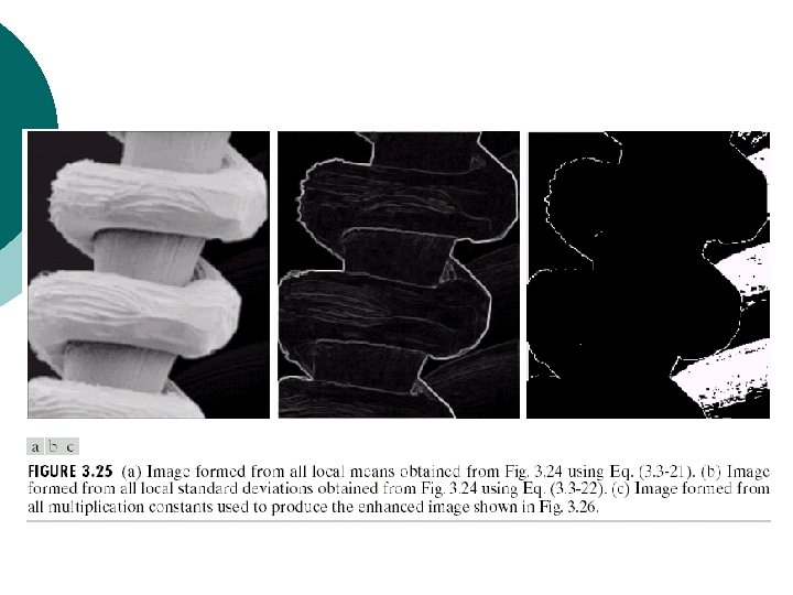
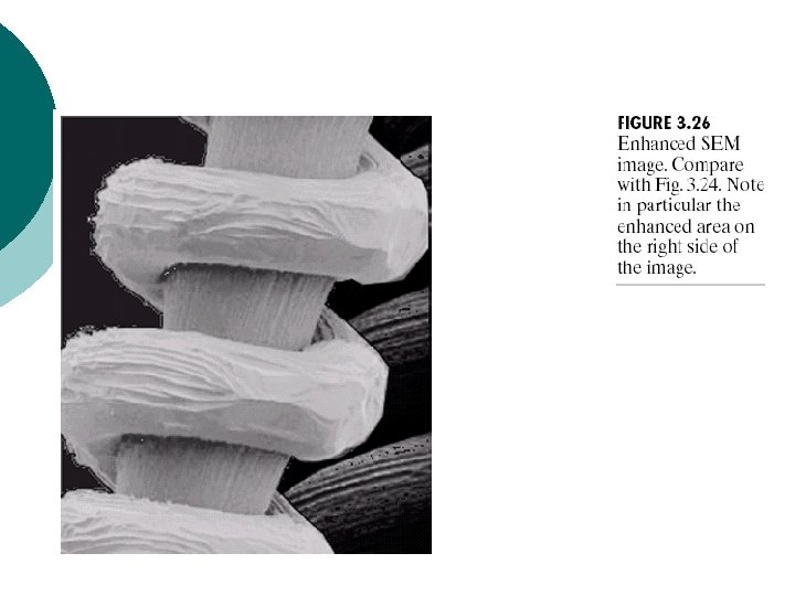
l l Global enhancement: The global mean and variance are measured over an entire image Local enhancement: The local mean and variance are used as the basis for making changes

l is the gray level at coordinates (s, t) in the neighborhood is the neighborhood normalized histogram component mean: l local variance l l

l l are specified parameters is the global mean is the global standard deviation Mapping

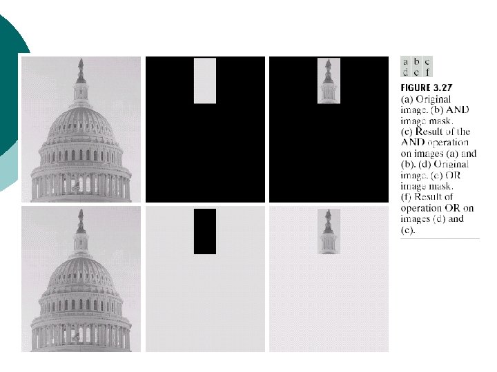
Enhancement Using Arithmetic/Logic Operations AND ¡ OR ¡ NOT ¡ Subtraction ¡ Addition ¡ Multiplication ¡ Division ¡

¡ Image subtraction l Enhancement of differences between images

l Mask mode radiography

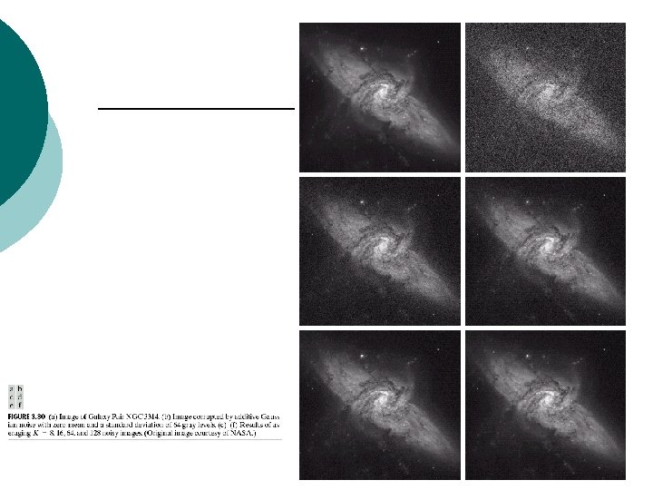
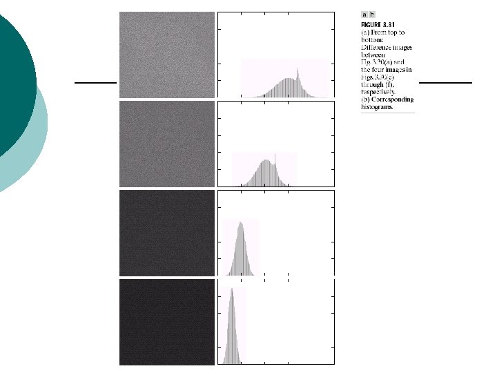
¡ Image Averaging l Averaging K different noisy images ,

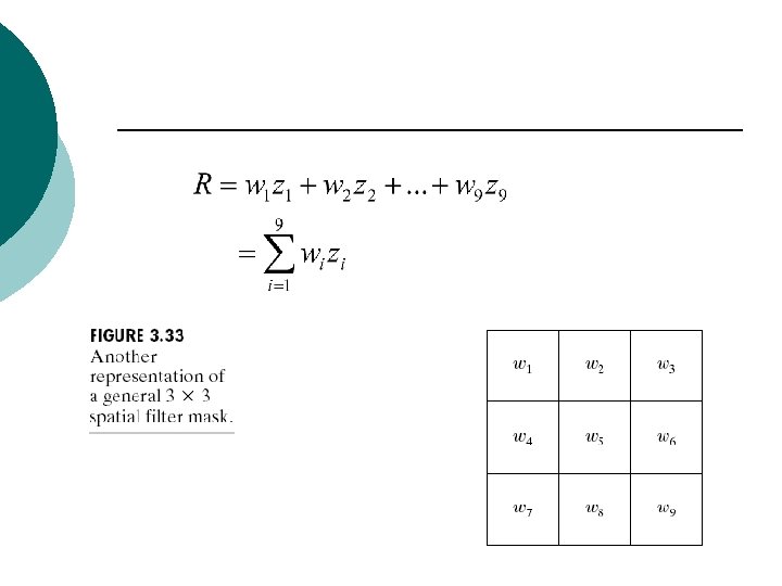
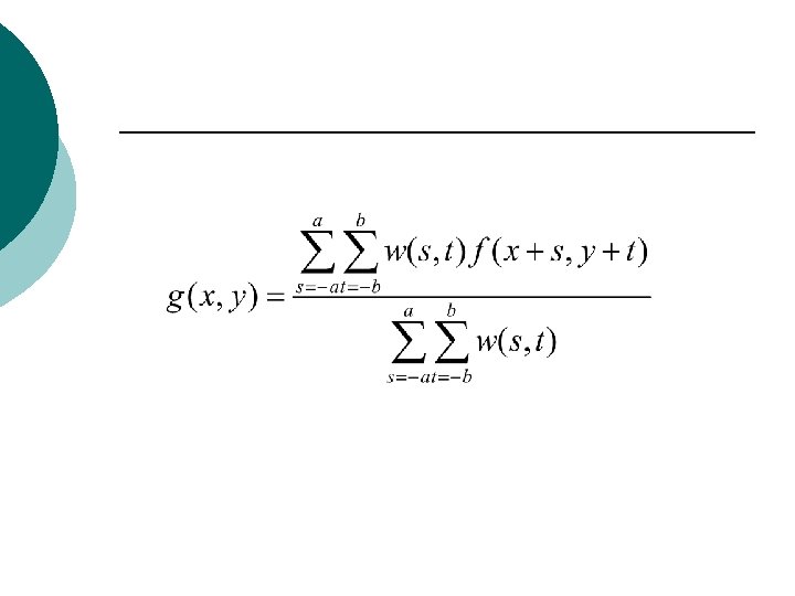
Basics of Spatial Filtering

l l Image size: Mask size: and

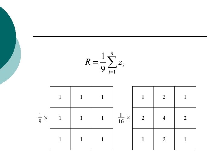
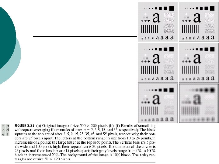
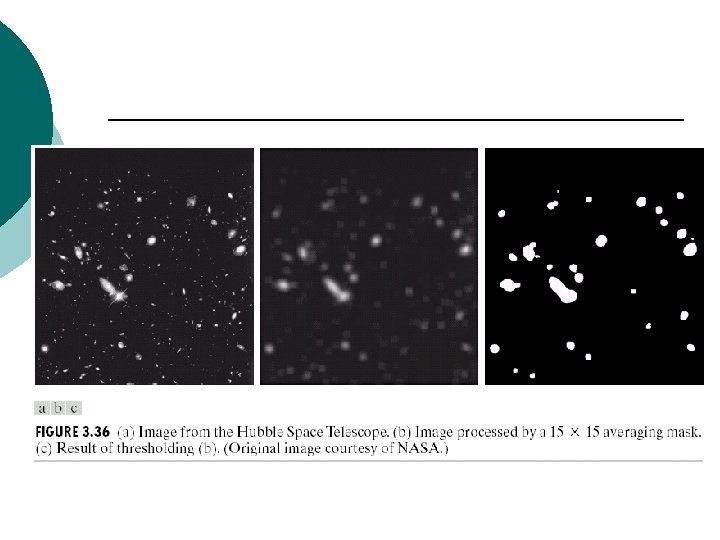
Smoothing Spatial Filters ¡ Smoothing l l l Noise reduction Smoothing of false contours Reduction of irrelevant detail

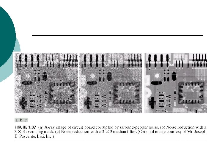
¡ Order-statistic filters l l median filter: Replace the value of a pixel by the median of the gray levels in the neighborhood of that pixel Noise-reduction

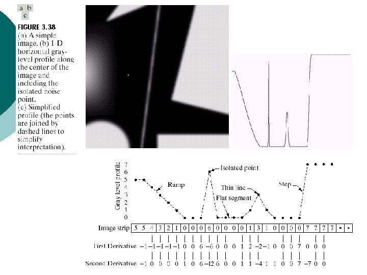
Sharpening Spatial Filters ¡ Foundation l The first-order derivative l The second-order derivative

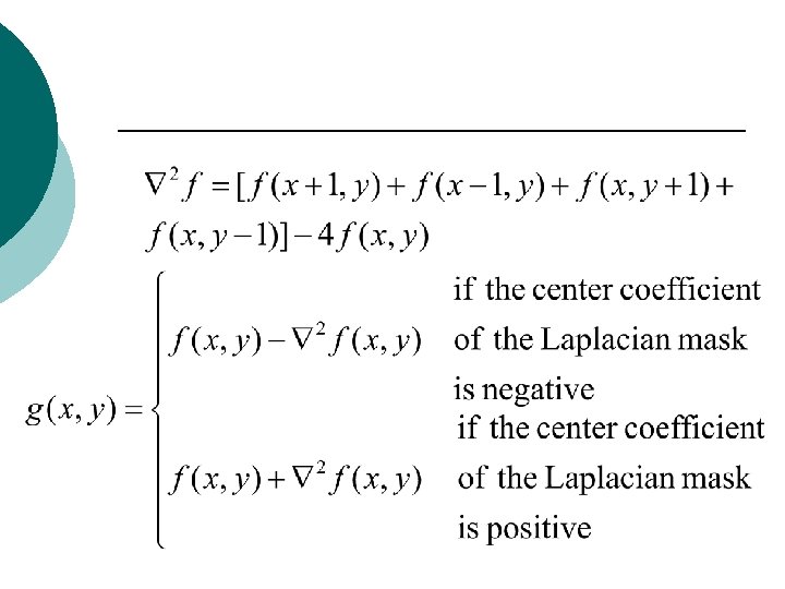
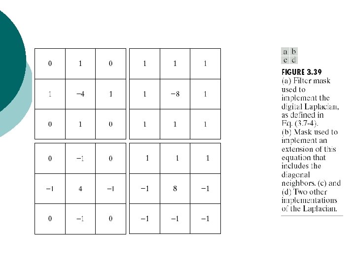
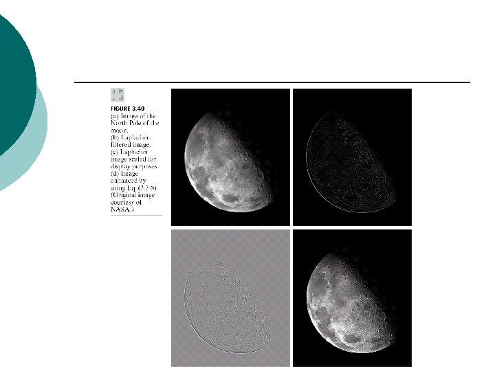
¡ Use of second derivatives for enhancement-The Laplacian l Development of the method

l Simplifications

¡ Unsharp masking and high-boost filtering l Unsharp masking ¡ ¡ Substract a blurred version of an image from the image itself : The image, blurred image : The

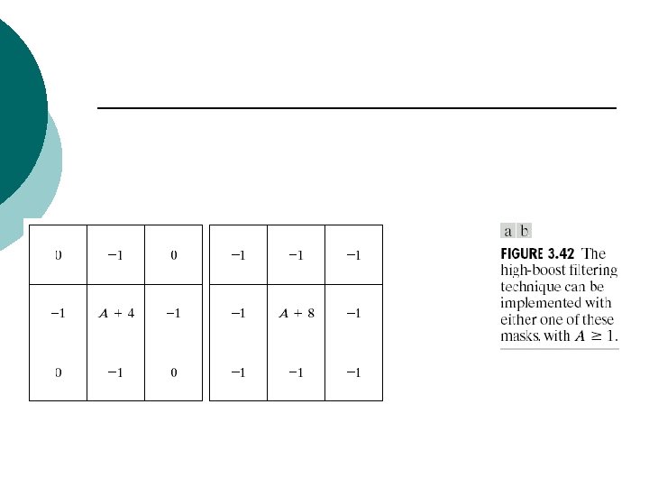
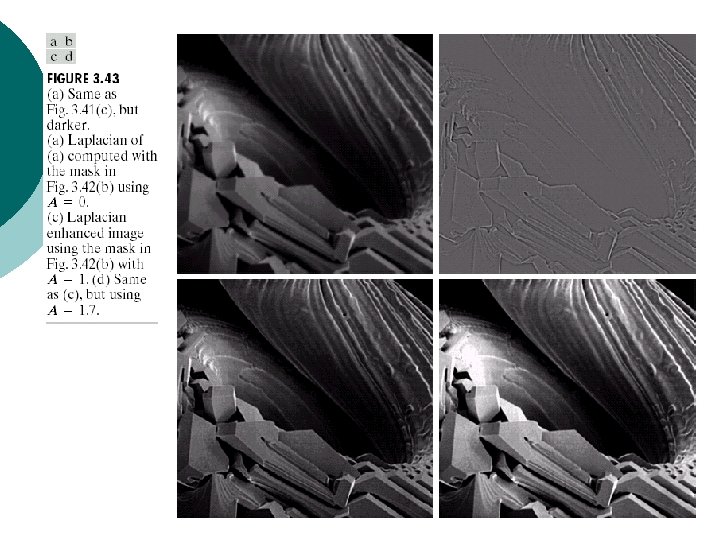
l High-boost filtering

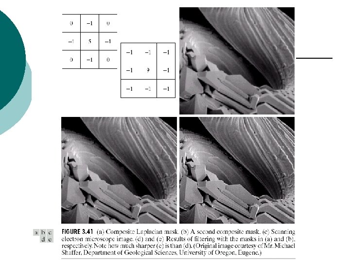
¡ Use the Laplacian as the sharpening filtering

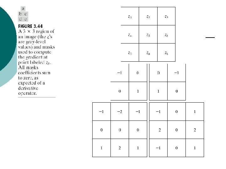
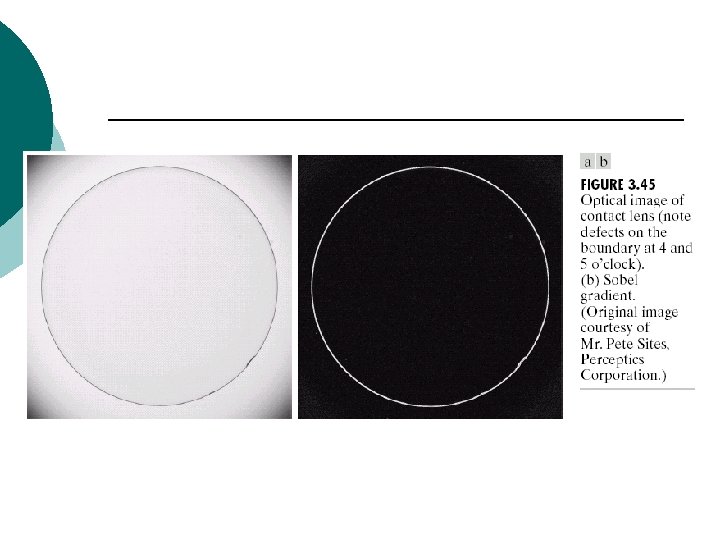
¡ Use of first derivatives for enhancement—The gradient

l The magnitude is rotation invariant (isotropic)

l Computing using cross differences, Roberts cross-gradient operators and

l Sobel operators ¡ A weight value of 2 is to achieve some smoothing by giving more importance to the center point

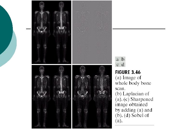
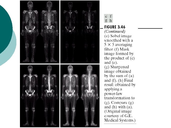
Combining Spatial Enhancement Methods ¡ An example l l Laplacian to highlight fine detail Gradient to enhance prominent edges Smoothed version of the gradient image used to mask the Laplacian image Increase the dynamic range of the gray levels by using a gray-level transformation

Example 1 ¡ ¡ ¡ Histogram Equalization (a) Write a computer program for computing the histogram of an image. (b) Implement the histogram equalization technique discussed in Section 3. 3. 1. (c) Download Fig. 3. 8(a) and perform histogram equalization on it. Fig 3. 08(a). bmp histo. c

Example 2 ¡ ¡ ¡ Arithmetic Operations Write a computer program capable of performing the four arithmetic operations between two images. This project is generic, in the sense that it will be used in other projects to follow. (See comments on pages 112 and 116 regarding scaling). In addition to multiplying two images, your multiplication function must be able to handle multiplication of an image by a constant. Fig 3. 08(a). bmp new 2. bmp arithmetic. c