Digital Image Processing Chapter 2 Digital Image Fundamentals

Digital Image Processing Chapter 2: Digital Image Fundamentals

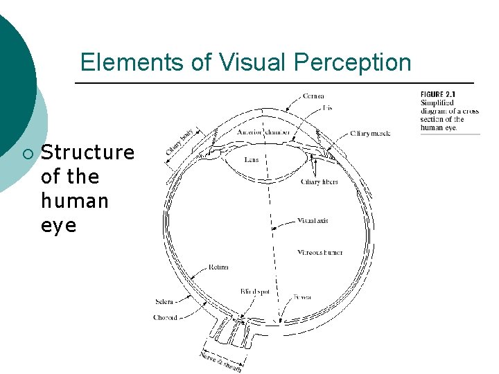
Elements of Visual Perception ¡ Structure of the human eye

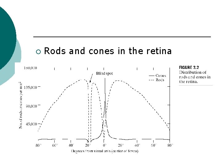
¡ Rods and cones in the retina

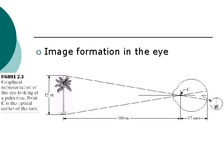
¡ Image formation in the eye

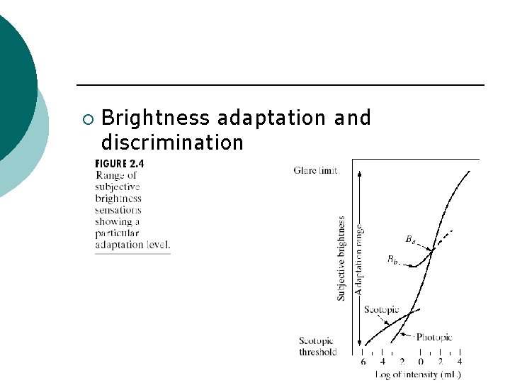
¡ Brightness adaptation and discrimination

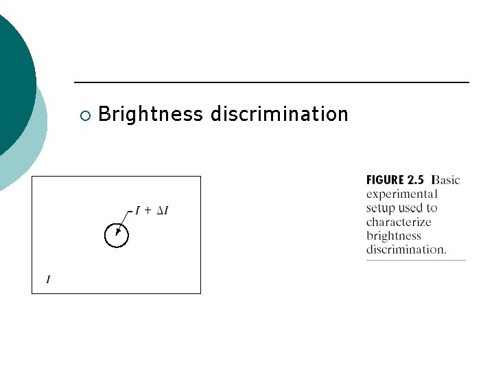
¡ Brightness discrimination

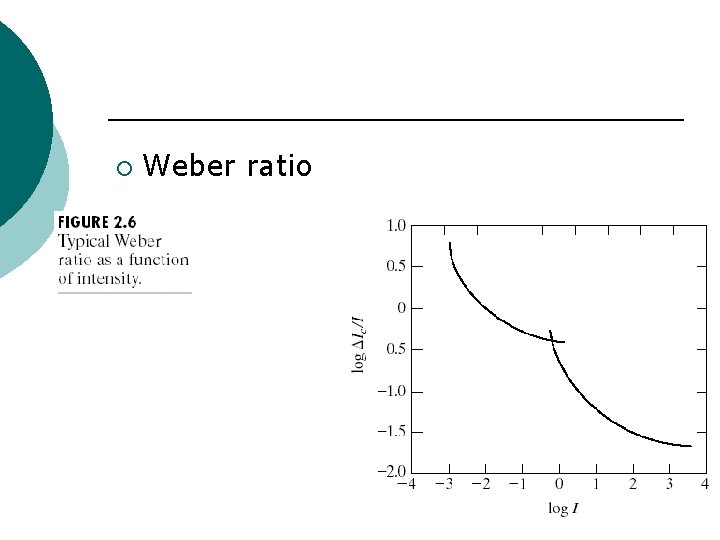
¡ Weber ratio

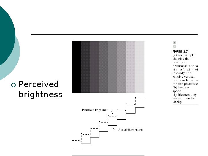
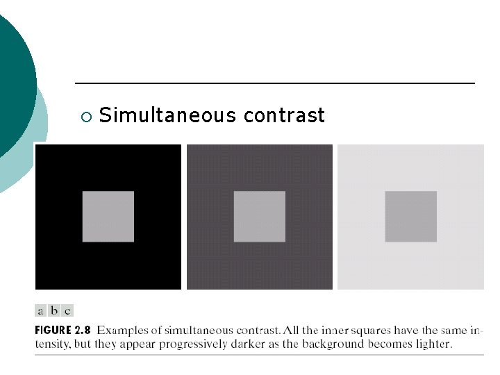
¡ Perceived brightness

¡ Simultaneous contrast

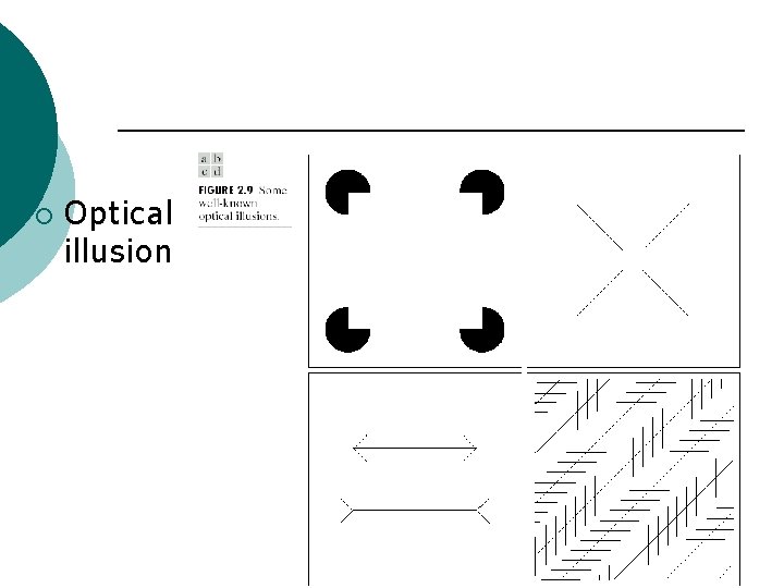
¡ Optical illusion

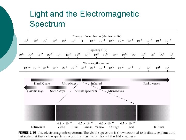
Light and the Electromagnetic Spectrum

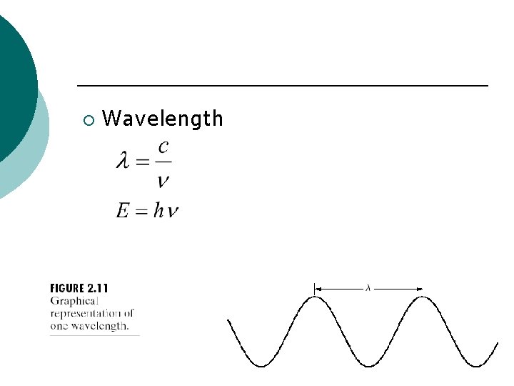
¡ Wavelength

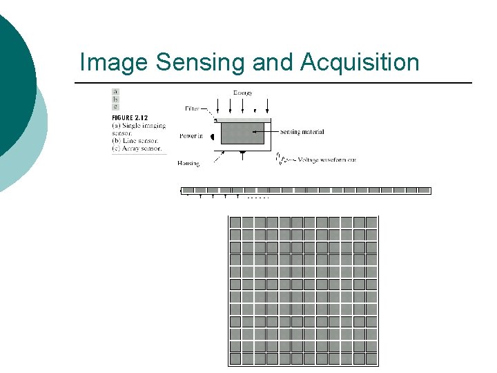
Image Sensing and Acquisition

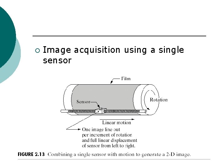
¡ Image acquisition using a single sensor

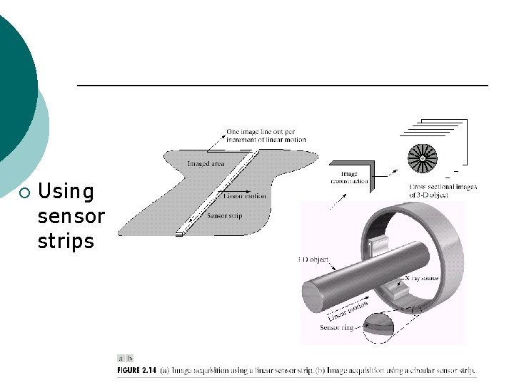
¡ Using sensor strips

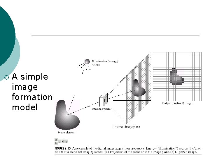
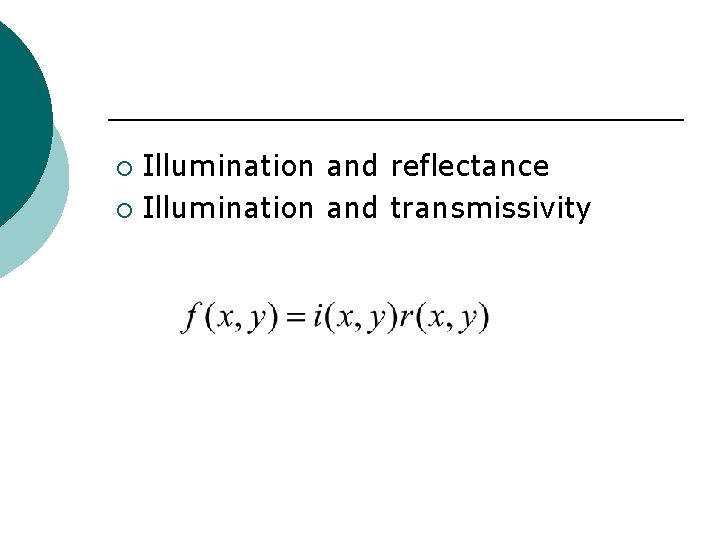
¡ A simple image formation model

Illumination and reflectance ¡ Illumination and transmissivity ¡

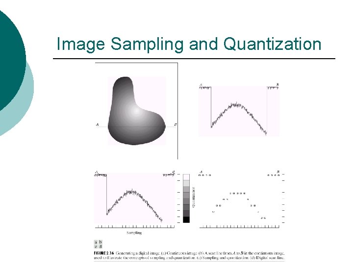
Image Sampling and Quantization

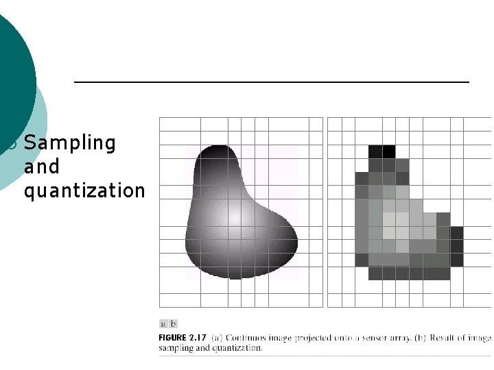
¡ Sampling and quantization

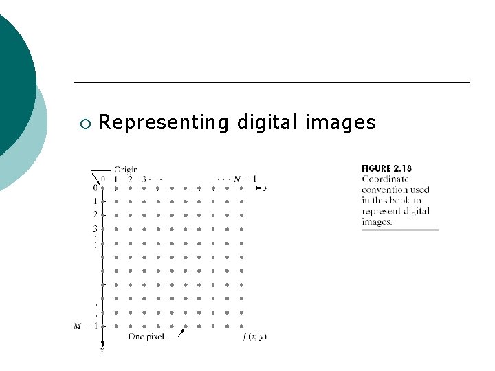
¡ Representing digital images

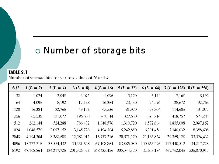
¡ Number of storage bits

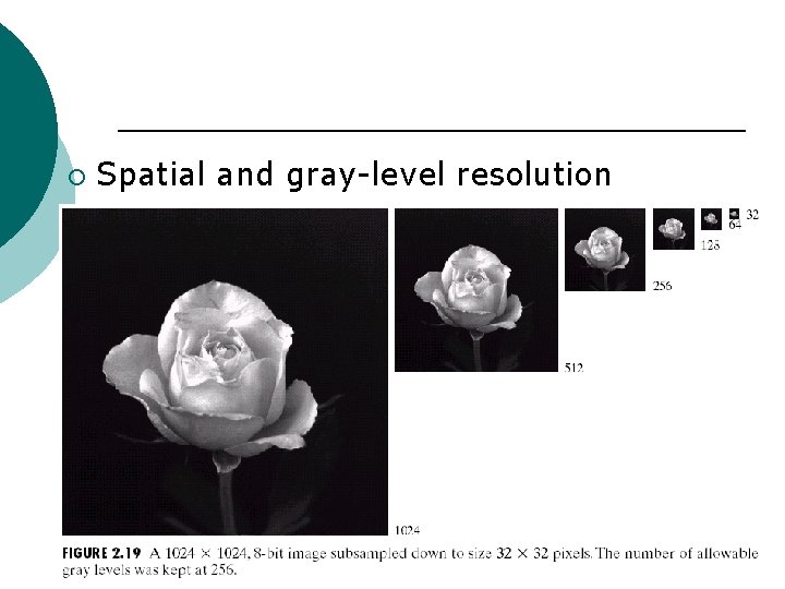
¡ Spatial and gray-level resolution

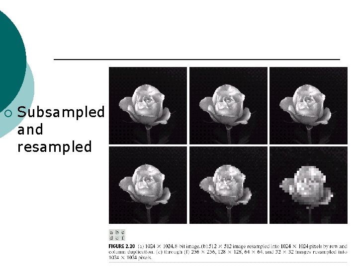
¡ Subsampled and resampled

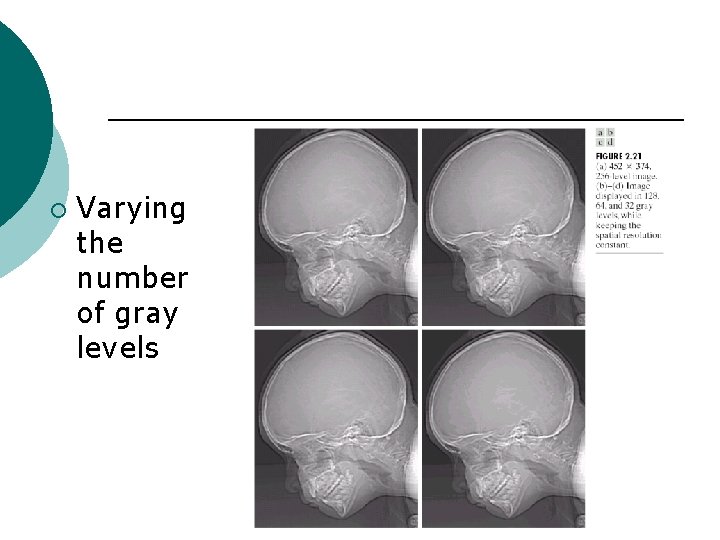
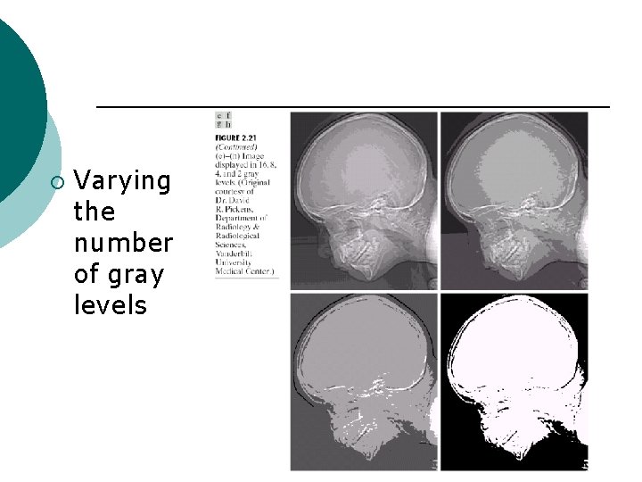
¡ Varying the number of gray levels

¡ Varying the number of gray levels

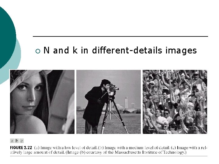
¡ N and k in different-details images

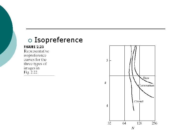
¡ Isopreference

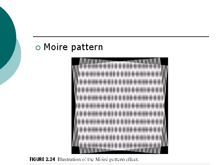
¡ Moire pattern

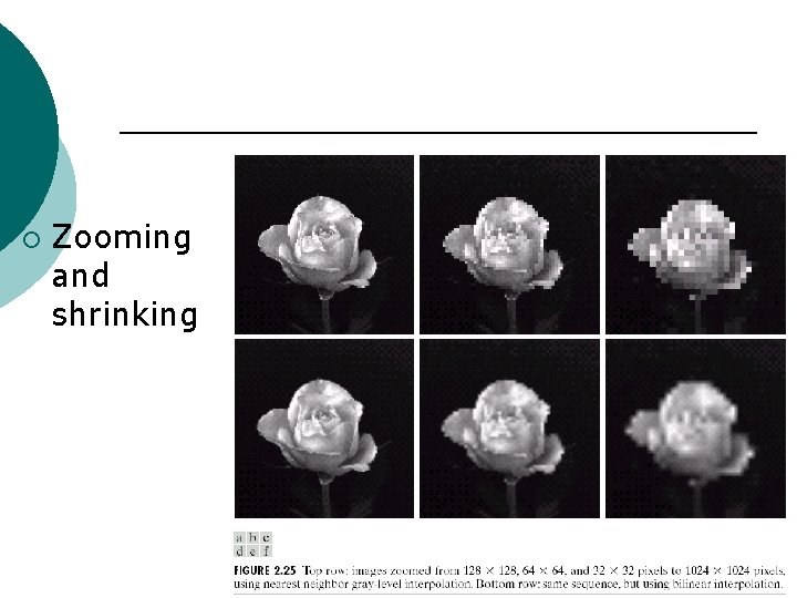
¡ Zooming and shrinking

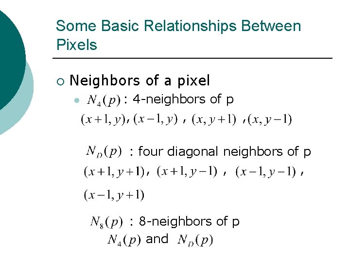
Some Basic Relationships Between Pixels ¡ Neighbors of a pixel l : 4 -neighbors of p , , , : four diagonal neighbors of p , , , : 8 -neighbors of p and

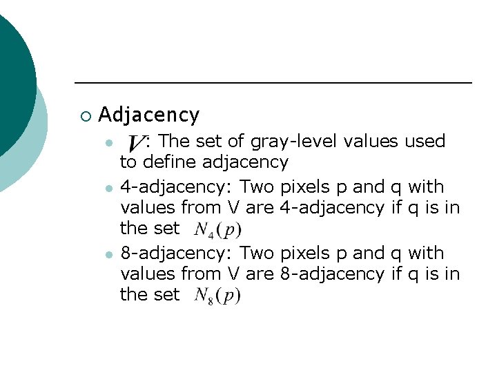
¡ Adjacency l l l : The set of gray-level values used to define adjacency 4 -adjacency: Two pixels p and q with values from V are 4 -adjacency if q is in the set 8 -adjacency: Two pixels p and q with values from V are 8 -adjacency if q is in the set

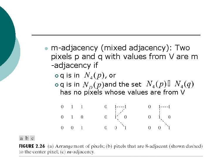
l m-adjacency (mixed adjacency): Two pixels p and q with values from V are m -adjacency if q is in , or ¡ q is in and the set has no pixels whose values are from V ¡

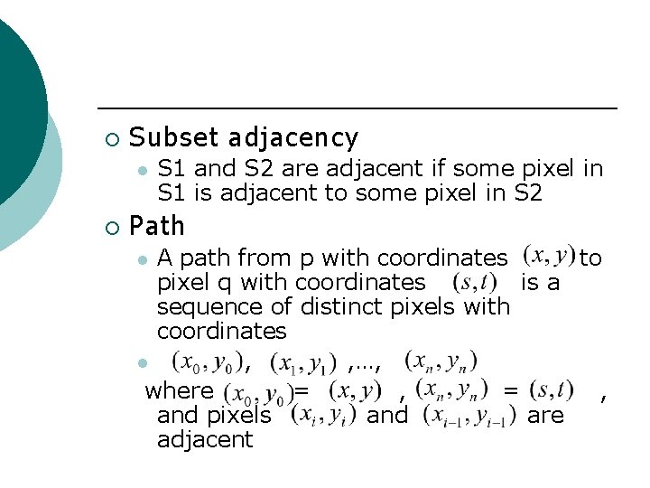
¡ Subset adjacency l ¡ S 1 and S 2 are adjacent if some pixel in S 1 is adjacent to some pixel in S 2 Path A path from p with coordinates to pixel q with coordinates is a sequence of distinct pixels with coordinates l , , …, where = , and pixels and are adjacent l

¡ Region l ¡ Boundary l ¡ We call R a region of the image if R is a connected set The boundary of a region R is the set of pixels in the region that have one or more neighbors that are not in R Edge l Pixels with derivative values that exceed a preset threshold

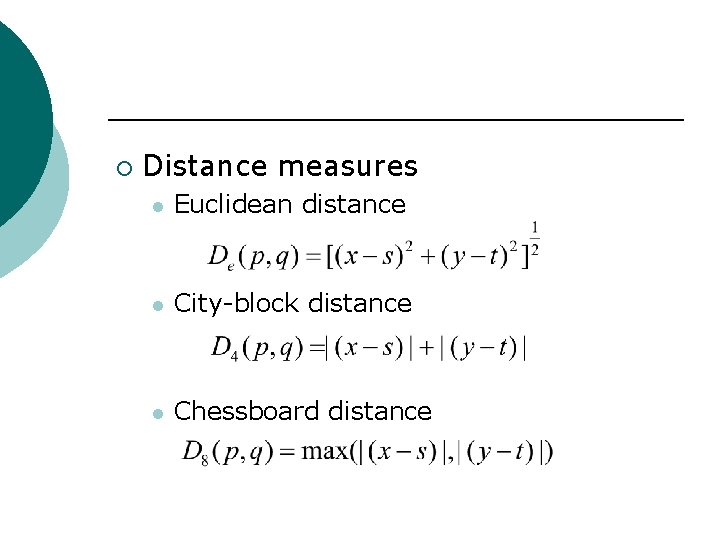
¡ Distance measures l Euclidean distance l City-block distance l Chessboard distance

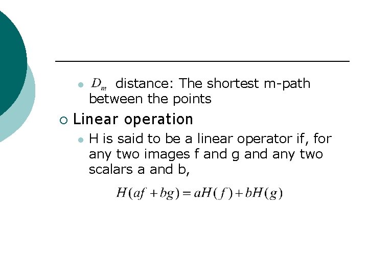
l ¡ distance: The shortest m-path between the points Linear operation l H is said to be a linear operator if, for any two images f and g and any two scalars a and b,

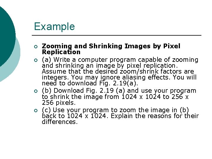
Example ¡ ¡ Zooming and Shrinking Images by Pixel Replication (a) Write a computer program capable of zooming and shrinking an image by pixel replication. Assume that the desired zoom/shrink factors are integers. You may ignore aliasing effects. You will need to download Fig. 2. 19(a). (b) Download Fig. 2. 19 (a) and use your program to shrink the image from 1024 x 1024 to 256 x 256 pixels. (c) Use your program to zoom the image in (b) back to 1024 x 1024. Explain the reasons for their differences.

http: //home. kimo. com. tw/abc 9250/ BMP_FILE. htm ¡ Fig 2. 19(a). bmp ¡ subsample. c ¡ resample. c ¡