Digital Image Processing 3 rd ed Chapter 9

Digital Image Processing, 3 rd ed. Chapter 9 Morphological Image Processing Dept. Computer Science & Engineering Hongtao Lu 3/12/2021

Outline • Preliminaries • Erosion and Dilation • Opening and Closing • The Hit-or-Miss Transformation • Some Basic Morphological Algorithms • Gray-Scale Morphology

Mathematical Morphology • Used to extract image components that are useful in the representation and description of region shape, such as § § § boundaries extraction skeletons convex hull morphological filtering thinning pruning

9. 1 Preliminaries • Sets in mathematical morphology represent objects in an image: § binary image (0 = white, 1 = black): the element of the set is the coordinates (x, y) of pixel belong to the object Z 2 § gray-scaled image: the element of the set is the coordinates (x, y) of pixel belong to the object and the gray levels Z 3

9. 1 Preliminaries • A: A set in Z 2 with elements of a = (a 1, a 2)

9. 1 Preliminaries • Operators by examples:

9. 1 Preliminaries • A: A set in Z 2 with elements of a = (a 1, a 2)

9. 1 Preliminaries • Reflection and Translation by examples: § Need for a reference point. (a) Translation of A by z. (b) Reflection of B.

9. 1 Preliminaries • Structuring elements (SEs) Figure 9. 2 First row: Examples of structuring elements. Second row: Structuring elements converted to rectangular arrays. The dots denote the centers of the SEs.

9. 1 Preliminaries Figure 9. 3 (a) A set (each shaded square is a member of the set). (b) A structuring element. (c) The set padded with background elements to form a rectangular array and provide a background border. (d) Structuring element as a rectangular array. (e) Set processed by the structuring element.

9. 2 Erosion and Dilation • Erosion With A and B as sets in Z 2, the erosion of A by B is defined as • Set B: A structural elements • Other banes: Shrink, Reduce

9. 2 Erosion and Dilation Figure 9. 4 (a) Set A. (b) Square structuring element, B. (c) Erosion of A by B, shown shaded. (d) Elongated structuring element. (e) Erosion of A by B using this element.

9. 2 Erosion and Dilation Figure 9. 5 Using erosion to remove image components. (a) A 486× 486 binary image of a wire-bond mask. (b)-(d) Image eroded using square structuring elements of sizes 11× 11, 15× 15, and 45× 45, respectively. The elements of the SEs were all 1 s.

9. 2 Erosion and Dilation • Dilation With A and B as sets in Z 2, the dilation of A by B is defined as • Set B: A structural elements • Relation to Convolution mask: § § Flipping Overlapping • Other names: Grow, Expand

9. 2 Erosion and Dilation Figure 9. 6 (a) Set A. (b) Square structuring element (the dot denotes the origin). (c) Dilation of A by B, shown shaded. (d) Elongated structuring element. (e) Dilation of A using this element.

• Application: Gap filling (a) Sample text of (b) Structuring element poor resolution with broken characters Dilation of (a) by (b)

9. 2 Erosion and Dilation • Dilation-Erosion Duality Remember: Similarly:

9. 3 Opening and Closing • Dilation expands and Erosion shrinks. • Opening: • Smooth contour • Break narrow isthmuses (Means: )ﺗﻨگﻪ • Remove thin protrusion • Closing • Smooth contour • Fuse narrow breaks, and long thin gulfs • Remove small holes, and fill gaps

9. 3 Opening and Closing • Opening: • An erosion followed by a dilation using the same structuring element for both operations. • Closing • A dilation followed by an erosion using the same structuring element for both operations.

9. 3 Opening and Closing • Opening Illustration Figure 9. 8 (a) Structuring element B “rolling” along the inner boundary of A (the dot indicates the origin of B). (b) Structuring element. (c) The heavy line is the outer boundary of the opening. (d) Complete opening (shaded). We did not shade A in (a) for clarity.

9. 3 Opening and Closing • Closing Illustration Figure 9. 9 (a) Structuring element B “rolling” on the outer boundary of set A. (b) The heavy line is the outer boundary of the closing. (c) Complete closing (shaded). We did not shade A in (a) for clarity.

Morphological opening and closing

• Medical Application Closing 5× 5 Opening 5× 5 Original Segmentation

9. 3 Opening and Closing • Opening and Closing Duality

9. 3 Opening and Closing • Opening Properties: • is a subset (subimage) of A. • If C is a subset of D, the is a subset of . • Multiple apply has no effect. • Closing Properties: • A is a subset (subimage) of • If C is a subset of D, then is a subset of • Multiple apply has no effect.

• Noise Reduction Opening Dilation of Opening Closing of Opening

9. 4 The Hit-or-Miss Transformation • Shape Detection • X-Y-X shape • X enclosed by W • B 1: Object related • B 2: Background related

Figure 9. 12 (a) Set A. (b) A window, W, and the local background of D with respect to W, (W – D). (c) Complement of A. (d) Erosion of A by D. (e) Erosion of Ac by (W – D). (f) Intersection of (d) and (e), showing the location of the origin of D, as desired.

9. 5 Some Basic Morphological Algorithms • Boundary Extraction (9. 5 -1) Figure 9. 13 (a) Set A. (b) Structuring element B. (c) A eroded by B. (d) Boundary, given by the set difference between A and its erosion.

9. 5 Some Basic Morphological Algorithms • Boundary Extraction Example Figure 9. 14 (a) A simple binary image, with 1 s represented in white. (b) Result of using Eq. (9. 5 -1) with the structuring element in Fig. 9. 13(b).

9. 5 Some Basic Morphological Algorithms • Hole (Region) Filling Start from p inside boundary. (9. 5 -2)

Figure 9. 15 Hole filling. (a) Set A (shown shaded). (b) Complement of A. (c) Structuring element B. (d) Initial point inside the boundary. (e)-(h) Various steps of Eq. (9. 5 -2). (i) Final result [union of (a) and (h)].

9. 5 Some Basic Morphological Algorithms • Hole (Region) Filling Example Figure 9. 16 (a) Binary image (the white dot inside one of the regions is the starting point for the hole-filling algorithm). (b) Result of filling that region. (c) Result of filling all holes.

9. 5 Some Basic Morphological Algorithms • Extraction of Connected Components Start from p belong to desired region. (9. 5 -3)

Figure 9. 17 Extracting connected components. (a) Structuring element. (b) Array containing a set with one connected component. (c) Initial array containing a 1 in the region of the connected component. (d)-(g) Various steps in the iteration of Eq. (9. 5 -3).

• Using connected components to detect foreign objects in packaged food.

9. 5 Some Basic Morphological Algorithms • Convex Hull of S • Smallest Convex set H, containing S • Define four basic structural elements, Bi, i = 1, 2, 3, 4

Figure 9. 19 (a) Structuring elements. (b) Set A. (c)-(f) Results of convergence with the structuring elements shown in (a). (g) Convex hull. (h) Convex hull showing the contribution of each structuring element. Converged: C C C

9. 5 Some Basic Morphological Algorithms • Shortcoming of previous algorithm: • Grow more than minimum required convex size. • Limit to vertical-horizontal expansion. Figure 9. 20 Result of limiting growth of the convex hull algorithm to the maximum dimensions of the original set of points along the vertical and horizontal directions.

9. 5 Some Basic Morphological Algorithms • Thinning Another approach: Repeat until convergence

Figure 9. 21 (a) Sequence of rotated structuring elements used for thinning. (b) Set A. (c) Results of thinning with the first element. (d)-(i) Results of thinning with the next seven elements. (j) Result of using the first four elements again. (l) Result after convergence. (m) Conversion to mconnectivity.

9. 5 Some Basic Morphological Algorithms • Thickening • Structural elements are as before Figure 9. 22 (a) Set A. (b) Complement of A. (c) Result of thinning the complement of A. (d) Thickened set obtained by complementing (c). (e) Final result, with no disconnected points.

9. 5 Some Basic Morphological Algorithms • Skeletons: S(A) (a) For z belong to S(A) and (D)z, the largest disk centered at z and contained in A, one cannot find a larger disk containing (D)z and included in A. The disk (D)z is called a maximum disk. (b) The disk (D)z touches the boundary of A at two or more different places.

9. 5 Some Basic Morphological Algorithms • Skeletons by example: Figure 9. 23 (a) Set A. (b) Various positions of maximum disks with centers on the skeleton of A. (c) Another maximum disk on a different segment of the skeleton of A. (d) Complete skeleton.

9. 5 Some Basic Morphological Algorithms • Formulations of Skeletons Reconstruction:

Implementation of computing the skeleton of a simple figure.

9. 5 Some Basic Morphological Algorithms • Pruning

Figure 9. 25 (a) Original image. (b) and (c) Structuring elements used for deleting end points. (d) Result of three cycles of thinning. (e) End points of (d). (f) Dilation of end points conditioned on (a). (g) Pruned image.

9. 5. 9 Morphological Reconstruction • Geodesic dilation • F: the marker image • G: the mask image • F and G are both binary image and The geodesic dilation of size 1 of F w. r. t G: Generally, ,

9. 5. 9 Morphological Reconstruction • Illustration of geodesic dilation

9. 5. 9 Morphological Reconstruction • Geodesic erosion The geodesic dilation of size 1 of F w. r. t G: Generally,

9. 5. 9 Morphological Reconstruction • Illustration of geodesic erosion

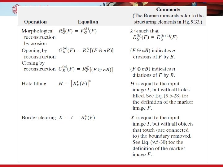
9. 5. 9 Morphological Reconstruction • Morphological reconstruction by dilation • The geodesic dilation of F w. r. t. G, iterated until stability, that is, with k such that

9. 5. 9 Morphological Reconstruction • Illustration of morphological reconstruction by dilation

9. 5. 9 Morphological Reconstruction • Morphological reconstruction by erosion • The geodesic erosion of F w. r. t. G, iterated until stability, that is, with k such that

9. 5. 9 Morphological Reconstruction • Sample applications • Opening by reconstruction restores exactly the shapes of the objects that remain after erosion. The opening by reconstruction of size n of an image F is defined as:

9. 5. 9 Morphological Reconstruction • Example of opening by reconstruction

9. 5. 9 Morphological Reconstruction • Sample applications • Filling holes A fully automated procedure based on morphological reconstruction. I(x, y): a binary image, form a marker image F: Then,

9. 5. 9 Morphological Reconstruction • Illustration of hole filling on a simple image

9. 5. 9 Morphological Reconstruction • A practical example of hole-filling

9. 5. 9 Morphological Reconstruction • Sample applications • Border clearing Use the original image as the mask and the following marker image: The border-Eclearing algorithm first computes the morphological reconstruction and then computes the difference:

9. 5. 9 Morphological Reconstruction • Example of border clearing Figure 9. 32 Border clearing. (a) Marker image. (b) Image with no objects touching the border.

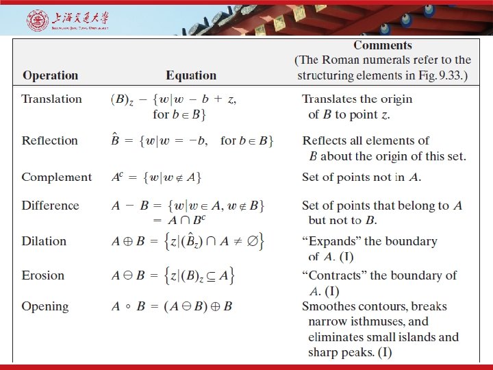
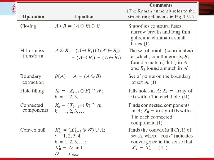
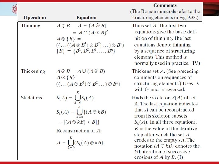
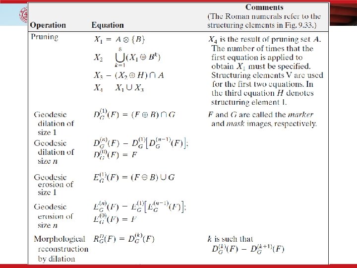
9. 5. 10 Summary of Morphological Operations on Binary Images Figure 9. 33 Five basic types of structuring elements used for binary morphology. The origin of each element is at its center and the ×’s indicate “don’t care” values.

9. 6 Gray-Scale Morphology • Extension to Gray-Level images: - f(x, y): the input image - b(x, y): a structuring element (a subimage function) - (x, y) are integers. - f and b are functions that assign a gray-level value (real number or real integer) to each distinct pair of coordinate (x, y)

9. 6 Gray-Scale Morphology • Extension to Gray-Level images Figure 9. 34 Nonflat and flat structuring elements, and corresponding horizontal intensity profiles through their center. All examples in this section are based on flat SEs.

9. 6 Gray-Scale Morphology • Erosion Condition (x+s) and (y+t) have to be in the domain of f and (x, y) have to be in the domain of b is similar to the condition in binary morphological erosion where the structuring element has to be completely contained by the set being eroded.

9. 6 Gray-Scale Morphology • Dilation Condition (x–s) and (y–t) have to be in the domain of f and (x, y) have to be in the domain of b is similar to the condition in binary morphological dilation where the two sets have to overlap by at least on element.

9. 6 Gray-Scale Morphology • Erosion and Dilation Duality where

9. 6 Gray-Scale Morphology • Illustration of gray-scale erosion and dilation Figure 9. 35 (a) A gray-scale X-ray image of size 448× 425 pixels. (b) Erosion using a flat disk SE with a radius of two pixels. (c) Dilation using the same SE.

9. 6 Gray-Scale Morphology • Opening • Closing • Opening and Closing Duality

9. 6 Gray-Scale Morphology Figure 9. 36 Opening and closing in one dimension. (a) Original 1 -D signal. (b) Flat structuring element pushed up underneath the signal. (c) Opening. (d) Flat structuring element pushed down along the top of the signal. (e) Closing.

9. 6 Gray-Scale Morphology • Opening-Closing Properties: - Opening: - Closing:

9. 6 Gray-Scale Morphology • Illustration of gray-scale erosion and dilation Figure 9. 37 (a) A gray-scale X-ray image of size 448× 425 pixels. (b) Opening using a disk SE with a radius of 3 pixels. (c) Closing using an SE of radius 5.

9. 6. 3 Some Basic Gray-Scale Morphological Algorithms • Smoothing: • Gradient: • Laplacian:

Figure 9. 38 (a) 566× 566 image of the Cygnus Loop supernova, taken in the X-ray band by NASA’s Hubble Telescope. (b)-(d) Results of performing opening and closing sequences on the original image with disk structuring elements of radii, 1, 3, and 5, respectively.

Figure 9. 39 (a) 512× 512 image of a head CT scan. (b) Dilation. (c) Erosion. (d) Morphological gradient, computed as the difference between (b) and (c).

9. 6. 3 Some Basic Gray-Scale Morphological Algorithms • Top-hat and bottom-hat transformations Combining image subtraction with openings and closings: Enhancing details in presence of shades

Figure 9. 40 Using the top-hat transformation for shading correction. (a) Original image of size 600× 600 pixels. (b) Thresholded image. (c) Image opened using a disk SE of radius 40. (d) Top-hat transformation (the image minus its opening). (e) Thresholded top-hat

9. 6. 3 Some Basic Gray-Scale Morphological Algorithms • Granulometry Figure 9. 41 (a) 531× 675 image of wood dowels. (b) Smoothed image. (c) -(f) Openings of (b) with disks of radii to 10, 235, and 30 pixels.

9. 6. 3 Some Basic Gray-Scale Morphological Algorithms • Granulometry Figure 9. 42 Differences in surface area as a function of SE disk radius, r. The two peaks are indicative of two dominant particle sizes in the image.

9. 6. 3 Some Basic Gray-Scale Morphological Algorithms • Textural segmentation

9. 6. 4 Gray-Scale Morphological Reconstruction • f: the marker image • g: the mask image • Both f and g are gray-scale images of the same size and f ≤ g. • Geodesic dilation of size 1 of f w. r. t. g: Generally, with

9. 6. 4 Gray-Scale Morphological Reconstruction • Geodesic erosion of size 1 of f w. r. t. g: Generally, with

9. 6. 4 Gray-Scale Morphological Reconstruction • The morphological reconstruction by dilation with k such that • The morphological reconstruction by erosion with k such that

9. 6. 4 Gray-Scale Morphological Reconstruction • The opening by reconstruction of size n of f: • The closing by reconstruction of size n of f:

Using morphological reconstruction to flatten a complex background.