Diffusion Tensor Estimation Method Robert Cox and Daniel

Diffusion Tensor Estimation Method Robert Cox and Daniel Glen Scientific and Statistical Computing Core NIMH

DTI Overview MRI imaging method that shows relative rates and directions of diffusion corresponding to flow principally along fiber tracts Applications for diseases involving white matter including perinatal brain injury, stroke, multiple sclerosis, tumors, …. Acquisition of MRI volume followed by at least six or more volumes (typically many more) with an additional gradient applied from non-collinear directions I(q) = J e –b(q) . D Where (q) = the image voxel intensity for each gradient q I(q) J = the ideal image intensity without applied gradient usually taken as J = I(0) (q) = “b-matrix” = g 2 G G d 2(D-d/3) for the qth encoding gradient b(q) i j g = 267. 5 rad/ms. m. T, D= time lag between starts of gradient, d = duration of gradient D = the Diffusion tensor, Diffusion in 6 principal directions, Dxx, Dxy, Dxz, Dyy, Dyz, Dzz ln(I(0) / I(q)) = b(q). D D = ln(I(0) / I(q) ) x b-1

Eigenvalue calculations DV=l. V Where D = diffusion tensor in a symmetric, square matrix form (3 x 3) V = the eigenvector, a vector corresponding to an orientation (3 x 1) l = the eigenvalue, a scalar constant For a 3 x 3 matrix, there are 3 sets of orthogonal eigenvector and eigenvalue solutions det(D – l. I) = 0 (D – l. I) V = 0 Solved with f 2 c converted eispack routine in AFNI using a tridiagonal reduction followed by a QL 2 solution for the eigenvalues and vectors

General Measures n Fractional Anisotropy (FA) FA =Ö (l 1 - l 2)2 + (l 1 - l 3)2 + (l 2 - l 3)2 Ö 2 Öl 12 + l 22 + l 32 n Lattice Index (LI) = S an. LIn / S an LIn = ~ n Mean Diffusivity l = (l 1 + l 2 + l 3) / 3

DWI, DT, Eigenvalue Samples DWI q 1 l 1 Dxx

DTI images Color coded EV 1 FA A-P green L-R red I-S blue

Negative Eigenvalues Skare, et. al, Mag. Res. Imaging, 18, 2000

Negative Eigenvalue Solutions Negative values more likely with increasing FA and with increasing noise (Skare, et al, Basser) n n n Calculate FA with negative eigenvalues reset to 0 (GE, Hopkins DTI Studio) Use another index, e. g. Lattice Anisotropy Index (Basser) Spatial smoothing of DWI images (Hahn, et al) Temporal smoothing with repeat experiments (Skare, et al) Calculate D, limiting D to positive definite matrix (Tschumperlé and Deriche, Mangin et al)

Direct Least Squares for D I(q) n Ø = Je –b(q) . D + noise Noise – Johnson noise, Eddy currents, motion including periodic beat of CSF with blood flow, partial volume effect Find the symmetric non-negative definite matrix D that minimizes the Error functional (cost function) E(D, J) = ½ Sq w(q) (J e –b(q). D 2 (q) -I ) Generally, estimate D, adjust through a gradient step to find new estimate for D until D converges. Construct gradient step to guarantee D is always positive definite (no negative eigenvalues).

Initial Estimate of D, D 0 n n n Estimate for D the traditional way and find eigenvalues, vectors too Limit eigenvalues to positive ones by setting l 2, l 3 eigenvalues to be at least 0. 2*l 1 Recompute D 0 = U L UT Where U = [u 1, u 2, u 3] matrix of eigenvectors L = diag(l 1, l 2, l 3)

Compute J (Ideal image voxel value) E(D, J) = ½ ¶E/¶J = S J = (S S w(q) (S (J e –b(q). D I(q) w(q) –b(q). D w(q) e e - I(q)) –b(q). D) – 2 b(q). D) 2 (q) -I ) / e –b(q). D

Modified Gradient Descent Gradient of E (error) with respect to D = F F = S w(q) (J e –b(q). D-I(q)) b(q) We want to change D to minimize E the fastest. From definition of gradient, ¶ D/¶ t = -F (we don’t use this) Where t is pseudo-time in the descent. But this doesn’t prevent D from becoming nonpositive definite, so instead …

Modified Gradient Descent ¶D/ ¶t = -(FD 2 + D 2 F) This can be shown to be the fastest descent while remaining positive definite We will do the descent with finite steps If ¶D/ ¶t = -(ND + DN) with N as a constant matrix, it can also be shown D(t + Dt) = e(-Dt. N) D(t) e(-Dt. N) Let N=FD and approximately constant over Dt step D(t + Dt) = e(-FDDt) D(t) e(-FDDt)

Modified Gradient Descent We can replace e-x with the Padé approximant (similar to a Taylor series expansion) e-x ~ (1 - x/2) / (1 + x/2) Similarly, for a matrix exponential, e-M ~ (I – ½ M) (I + ½ M)-1 If we let H± = I ± ½ Dt FD Then D(t + Dt) = H-(Dt) H+(Dt)-1 D(t) H+(Dt)-1 H-(Dt) D(t + Dt) = A(Dt) D(t) A(Dt)T where A = H- H+ , which will always be symmetric and positive definite

Dt, pseudo-time step size calculation Initial Dt conservatively estimated Dt 0 = 0. 01 S |D 0| / S |G| where G = FD 2 + D 2 F Start with initial calculation of J, E(D, J) (Cost function) Take trial step of Dt 0 D(t + Dt) = A(Dt) D(t) A(Dt)T Recalculate J and E(D, J) If the new E(D, J) is less than the previous E(D, J), use this time step

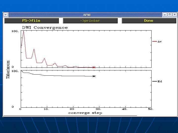
Modified Gradient Descent Algorithm n n n Compute D traditional linear way Compute eigenvalues and adjust Compute D based on new eigenvalues Calculate Ed = E(D, J) error Compute Initial Dt Take trial steps until convergence • Find acceptable trial step Dt that gives lower Ed by halving the initial Dt up to 10 times • Try step size of 2 Dt, ½Dt. Compute corresponding Ed, D for each and pick the Dt, D that gives the lowest Ed. Use Dt as the initial time step in the next convergence loop • Test convergence (starting with second step) n n S |Dnew – Dold| / S |Dnew| < 10 -4 Optionally recompute convergence loop with new weight factors

Weight Factor Computation The initial weight factors were all set to 1 n Recompute weight factors to downweight data points (gradients) that don’t fit well (outliers) n Compute residual at each gradient level from (0. . n) as. rq = J e –b(q) D-I(q) Estimate Std. Dev. as s = [1/Nq S rq 2] ½ wq = [1 / sqrt( 1+ (rq /s)2)] * Nq / S [1 / sqrt( 1+ (rq /s)2)] n

FA - non-linear FA - linear

Ratio of final E(D, J) to E(D, J) at t=0

Number steps to convergence without reweighting

Usage: 3 d. DWIto. DT [options] gradient-file dataset Computes 6 principle direction tensors from multiple gradient vectors and corresponding DTI image volumes. The program takes two parameters as input : a 1 D file of the gradient vectors with lines of ASCII floats Gxi, Gyi, Gzi. Only the non-zero gradient vectors are included in this file (no G 0 line). a 3 D bucket dataset with Np+1 sub- briks where the first sub-brik is the volume acquired with no diffusion weighting. Options: -automask = mask dataset so that the tensors are computed only for high-intensity (presumably brain) voxels. The intensity level is determined the same way that 3 d. Clip. Level works. -max_iter_rw n = max number of iterations after reweighting (Default=5) values can range from 1 to any positive integer less than 101. -eigs = compute eigenvalues, eigenvectors and fractional anisotropy in sub-briks 6 -18. Computed as in 3 d. DTeig -debug_briks = add sub- briks with Ed (error functional), Ed 0 (original error) and number of steps to convergence -cumulative_wts = show overall weight factors for each gradient level May be useful as a quality control -nonlinear = compute iterative solution to avoid negative eigenvalues. This is the default method. -verbose nnnnn = print convergence steps every nnnnn voxels that survive to convergence loops (can be quite lengthy) -linear = compute simple linear solution -drive_afni = show convergence graphs every nnnnn voxels that survive to convergence loops. AFNI must have NIML communications on (afni -niml). -reweight = recompute weight factors at end of iterations and restart -max_iter n = maximum number of iterations for convergence (Default=10) values can range from -1 to any positive integer less than 101. A value of -1 is equivalent to the linear solution. A value of 0 results in only the initial estimate of the diffusion tensor solution adjusted to avoid negative eigenvalues. Example: 3 d. DWIto. DTnoise -prefix rw 01 - automask -reweight max_iter 10 - max_iter_rw 10 tensor 25. 1 D grad 02+orig. The output is a 6 sub-brick bucket dataset containing Dxx, Dxy, Dxz, Dyy, Dyz, Dzz. Additional sub-briks may be appended with the - eigs and -debug_briks options. These results are appropriate as the input to the 3 d. DTeig program.

Other Methods Comparison n Tschumperlé and Deriche, Variational Framework • Simultaneous spatial smoothing • Complicated cost function versus x 2 Y(ln (I(0)/I(q)) - gk. T D gk) + a f (|ÑD|) where Y(s) = log(1+s 2) and f(s) = sqrt(1+s 2) We use Y(s) = s 2, a = 0 (no spatial contribution) • Slightly more complicated gradient function n G = (F+FT)D 2 + D 2 (F+FT) • Linearized with ln(I(0) / I(q)) versus non-linear relationship, I(q) = J e –b(q). D + noise • No reweighting n Mangin, et al, Robust Tensor Estimation • Cost function, Geman-Mc. Lure M-estimator, made to remove outliers, ei 2 / (ei 2+C 2) where C=1. 48 mediani |ei| (we use reweighting) • Similar to traditional method, does not enforce positive definiteness on D

Future Directions n n n Create and show fiber tracts in SUMA and AFNI Test model with computed DWI and artificial noise Add other indices (Lattice Index, Mean diffusivity, …) Refine model and algorithm Respond to AFNI user requests

Acknowledgements n n n Rick Reynolds Rich Hammett Ziad Saad Peter Basser Wolfgang Gaggl, Fernanda Tovar-Moll