Diffusion of Networking Technologies ISP BIRS workshop 2013
Diffusion of Networking Technologies ISP BIRS workshop 2013 Sharon Goldberg Boston University Princeton University Zhenming Liu Princeton University

Diffusion in social networks: Linear Threshold Model [Kempe Kleinberg Tardos’ 03, Morris’ 01, Granovetter’ 78] A node’s utility depends only on its neighbors! I’ll adopt the innovation if θ of my friends do! θ=1 θ=2 θ=3 θ=4 θ=6 Optimization problem [KKT’ 03]: Given the graph and thresholds, what is the smallest seedset that can cause the entire network to adopt? Seedset: A set of nodes that can kick off the process. Marketers, policy makers, and spammers can target them as early adopters! What if the innovation is a networking technology (e. g. IPv 6, Secure BGP, Qo. S, etc) And the graph is the network?
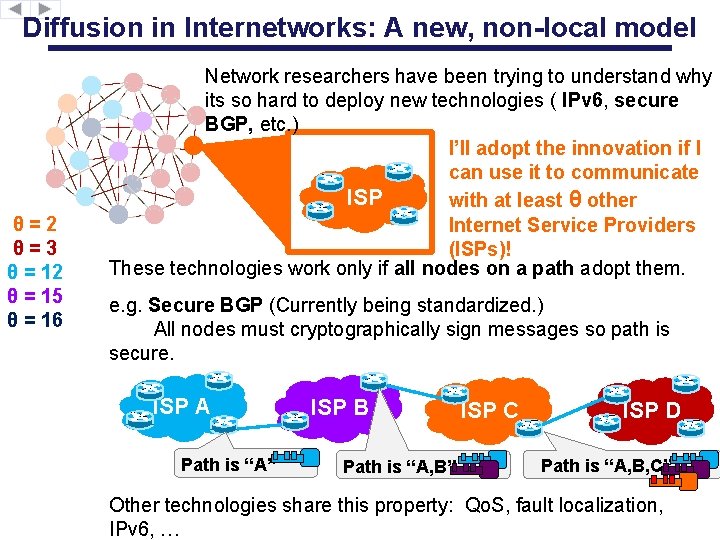
Diffusion in Internetworks: A new, non-local model θ=2 θ=3 θ = 12 θ = 15 θ = 16 Network researchers have been trying to understand why its so hard to deploy new technologies ( IPv 6, secure BGP, etc. ) I’ll adopt the innovation if I can use it to communicate ISP with at least θ other Internet Service Providers (ISPs)! These technologies work only if all nodes on a path adopt them. e. g. Secure BGP (Currently being standardized. ) All nodes must cryptographically sign messages so path is secure. ISP A Path is “A” ISP B Path is “A, B” ISP C ISP D Path is “A, B, C” Other technologies share this property: Qo. S, fault localization, IPv 6, …
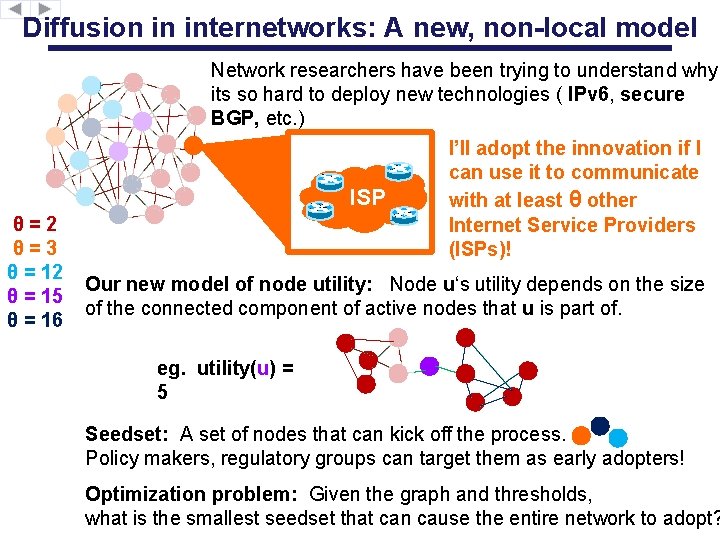
Diffusion in internetworks: A new, non-local model Network researchers have been trying to understand why its so hard to deploy new technologies ( IPv 6, secure BGP, etc. ) ISP θ=2 θ=3 θ = 12 θ = 15 θ = 16 I’ll adopt the innovation if I can use it to communicate with at least θ other Internet Service Providers (ISPs)! Our new model of node utility: Node u‘s utility depends on the size of the connected component of active nodes that u is part of. eg. utility(u) = 5 Seedset: A set of nodes that can kick off the process. Policy makers, regulatory groups can target them as early adopters! Optimization problem: Given the graph and thresholds, what is the smallest seedset that can cause the entire network to adopt?
Interpretation of the model • Diffusion of innovation in “traditional” social science literature (e. g. [Bass’ 69], [Katz & Shapiro’ 85]) – The utility of adopting a new technology depends on network externalities, i. e. the number of nodes that adopt the same product. – But no network structure is in the picture. • Social influence for viral marketing ([Kempe, Kleinberg, Tardos’ 03] and related works) – The network structure is explicitly given. – The utility of adoption depends only on a node’s direct neighbors. • This work: – “Interpolates” the above two cases: – Network is explicitly given. – Utility is non-local.

Social networks: Local influence I’ll adopt the innovation if θ of my friends do! θ=1 θ=2 θ=3 θ=4 θ=6 vs. Internetworks: Non-local influence ISP I’ll adopt the innovation if I am part of a connected component containing at least θ other ISPs!
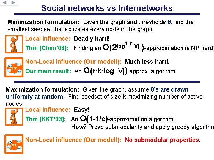
Social networks vs Internetworks Minimization formulation: Given the graph and thresholds θ, find the smallest seedset that activates every node in the graph. Local influence: Deadly hard! 1 -ε|V| log Thm [Chen’ 08]: Finding an O(2 )-approximation is NP hard. Non-Local influence (Our model!): Much less hard. ISP Our main result: An O(r∙k∙log |V|) approx algorithm Maximization formulation: Given the graph, assume θ’s are drawn uniformly at random. Find seedset of size k maximizing number of active nodes. Local influence: Easy! Thm [KKT’ 03]: An O(1 -1/e)-approximation algorithm. How? Prove submodularity and apply greedy algorithm Non-Local influence (Our model!): No submodular properties. ISP
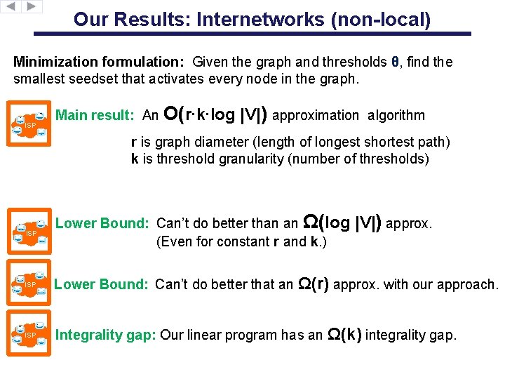
Our Results: Internetworks (non-local) Minimization formulation: Given the graph and thresholds θ, find the smallest seedset that activates every node in the graph. ISP Main result: An O(r∙k∙log |V|) approximation algorithm r is graph diameter (length of longest shortest path) k is threshold granularity (number of thresholds) ISP Lower Bound: Can’t do better than an Ω(log (Even for constant r and k. ) |V|) approx. ISP Lower Bound: Can’t do better that an Ω(r) approx. with our approach. ISP Integrality gap: Our linear program has an Ω(k) integrality gap.
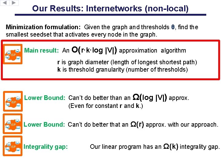
Our Results: Internetworks (non-local) Minimization formulation: Given the graph and thresholds θ, find the smallest seedset that activates every node in the graph. ISP Main result: An O(r∙k∙log |V|) approximation algorithm r is graph diameter (length of longest shortest path) k is threshold granularity (number of thresholds) ISP Lower Bound: Can’t do better than an Ω(log (Even for constant r and k. ) |V|) approx. ISP Lower Bound: Can’t do better that an Ω(r) approx. with our approach. ISP Integrality gap: Our linear program has an Ω(k) integrality gap.
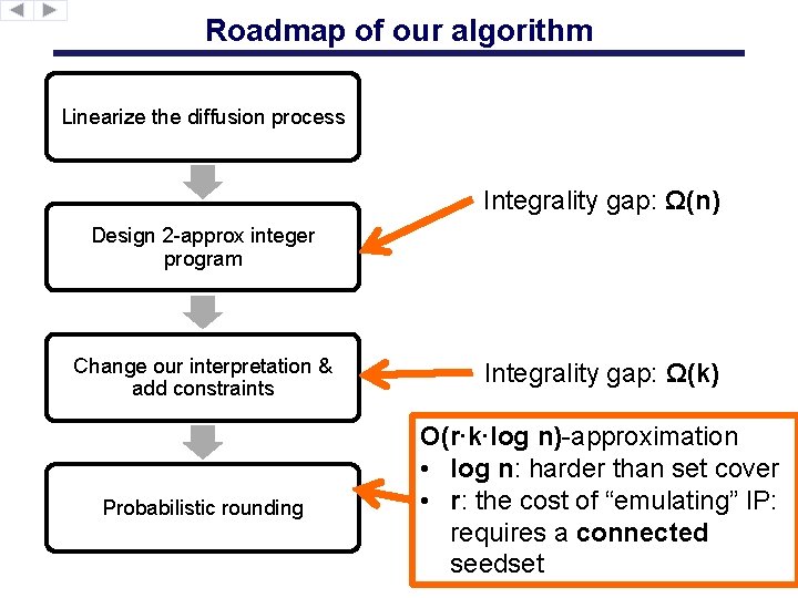
Roadmap of our algorithm Linearize the diffusion process Integrality gap: Ω(n) Design 2 -approx integer program Change our interpretation & add constraints Integrality gap: Ω(k) Probabilistic rounding O(r∙k∙log n)-approximation • log n: harder than set cover • r: the cost of “emulating” IP: requires a connected seedset
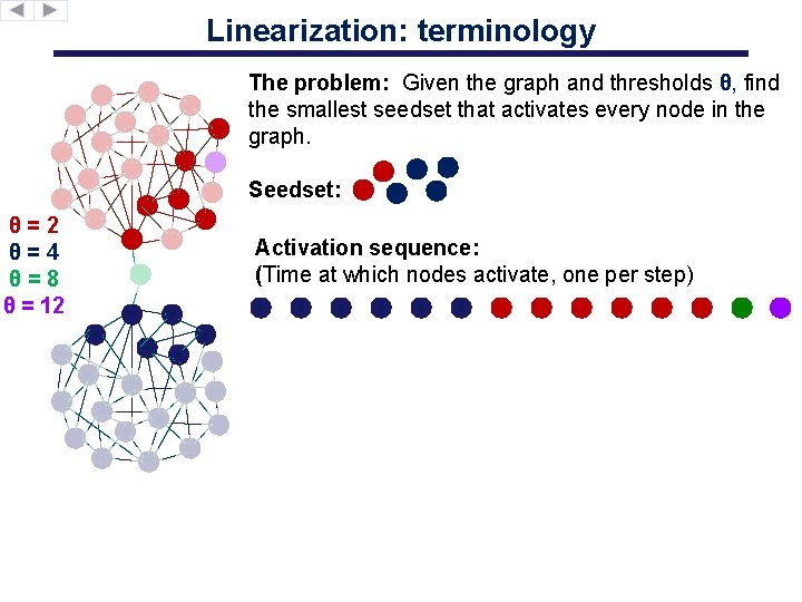
Linearization: terminology The problem: Given the graph and thresholds θ, find the smallest seedset that activates every node in the graph. Seedset: θ=2 θ=4 θ=8 θ = 12 Activation sequence: (Time at which nodes activate, one per step)
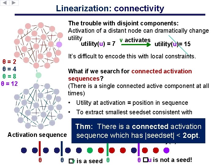
Linearization: connectivity The trouble with disjoint components: Activation of a distant node can dramatically change utility v activates utility(u) = 7 utility(u)= 15 It’s difficult to encode this with local constraints. θ=2 θ=4 θ=8 θ = 12 What if we search for connected activation sequences? (There is a single connected active component at all times) • Utility at activation = position in sequence • To extract smallest seedset consistent with sequence: Thm: There. Just is acheck connected if t > θ ! activation Activation sequence which has |seedset| < 2 opt. utility(v) < θ utility(u) = 15 > θ θ θ �v is a seed θ θ �u is not a seed!
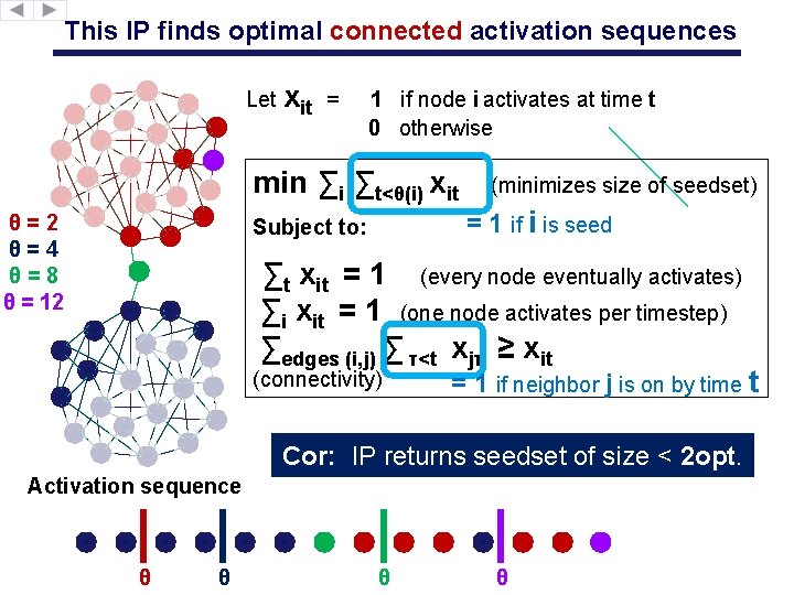
This IP finds optimal connected activation sequences Let xit = 1 if node i activates at time t 0 otherwise min ∑i ∑t<θ(i) xit θ=2 θ=4 θ=8 θ = 12 Subject to: (minimizes size of seedset) = 1 if i is seed ∑t xit = 1 (every node eventually activates) ∑i xit = 1 (one node activates per timestep) ∑edges (i, j) ∑ τ<t xjτ ≥ xit (connectivity) = 1 if neighbor j is on by time t Cor: IP returns seedset of size < 2 opt. Activation sequence θ θ
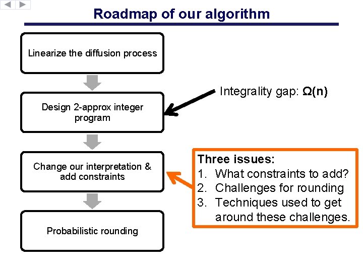
Roadmap of our algorithm Linearize the diffusion process Integrality gap: Ω(n) Design 2 -approx integer program Change our interpretation & add constraints Probabilistic rounding Three issues: 1. What constraints to add? 2. Challenges for rounding 3. Techniques used to get around these challenges.
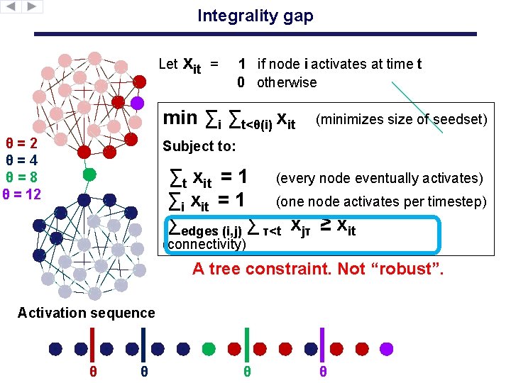
Integrality gap Let xit = 1 if node i activates at time t 0 otherwise min ∑i ∑t<θ(i) xit θ=2 θ=4 θ=8 θ = 12 (minimizes size of seedset) Subject to: ∑t xit = 1 (every node eventually activates) ∑i xit = 1 (one node activates per timestep) ∑edges (i, j) ∑ τ<t xjτ ≥ xit (connectivity) A tree constraint. Not “robust”. Activation sequence θ θ
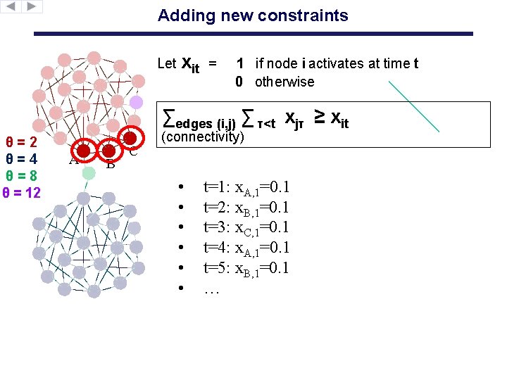
Adding new constraints Let xit = 1 if node i activates at time t 0 otherwise ∑edges (i, j) ∑ τ<t xjτ ≥ xit θ=2 θ=4 θ=8 θ = 12 A B C (connectivity) • • • t=1: x. A, 1=0. 1 t=2: x. B, 1=0. 1 t=3: x. C, 1=0. 1 t=4: x. A, 1=0. 1 t=5: x. B, 1=0. 1 …
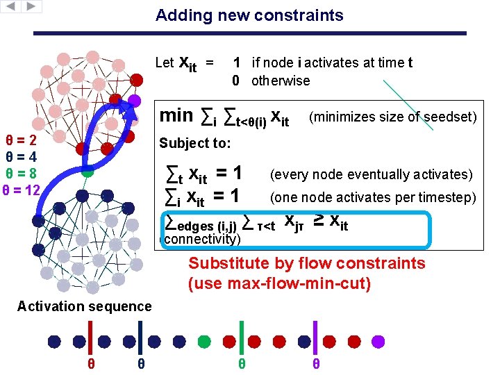
Adding new constraints Let xit = 1 if node i activates at time t 0 otherwise min ∑i ∑t<θ(i) xit θ=2 θ=4 θ=8 θ = 12 (minimizes size of seedset) Subject to: ∑t xit = 1 (every node eventually activates) ∑i xit = 1 (one node activates per timestep) ∑edges (i, j) ∑ τ<t xjτ ≥ xit (connectivity) Substitute by flow constraints (use max-flow-min-cut) Activation sequence θ θ
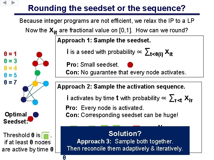
Rounding the seedset or the sequence? Because integer programs are not efficient, we relax the IP to a LP Now the xit are fractional value on [0, 1]. How can we round? Approach 1: Sample the seedset. i is a seed with probability ∝ ∑t<θ(i) xit θ=1 θ=3 θ=4 θ=5 θ=7 Pro: Small seedset. Con: No guarantee that every node activates. Approach 2: Sample the activation sequence. i activates by time t with probability ∝ ∑τ<t xiτ Pro: Every node is activated. Con: Corresponding seedset can be huge! Optimal Seedset: Necessary seedset: Approach 3: Sample both together. Then & iteratively. θ reconcile θ them θ adaptively θ � � �Solution? Threshold θ is. if at least θ nodes are active by time θ � θ
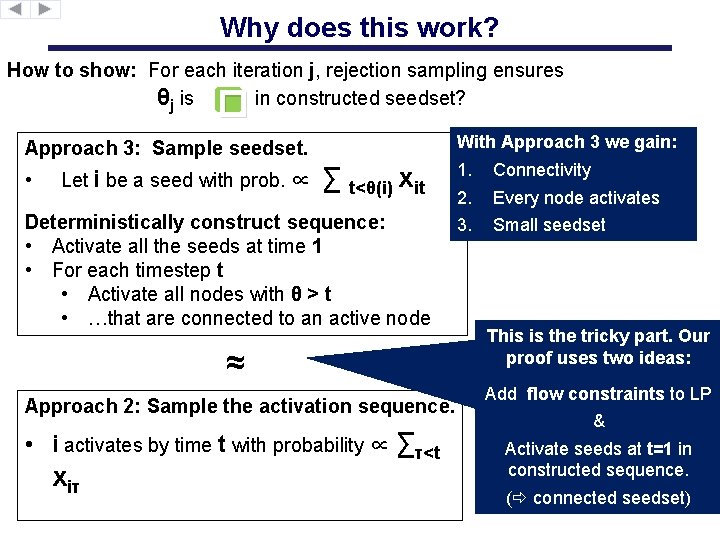
Why does this work? How to show: For each iteration j, rejection sampling ensures θj is in constructed seedset? � Approach 3: Sample seedset. • Let i be a seed with prob. ∝ ∑ t<θ(i) xit Deterministically construct sequence: • Activate all the seeds at time 1 • For each timestep t • Activate all nodes with θ > t • …that are connected to an active node ≈ Approach 2: Sample the activation sequence. • i activates by time t with probability ∝ ∑τ<t xiτ With Approach 3 we gain: 1. 2. 3. Connectivity Every node activates Small seedset This is the tricky part. Our proof uses two ideas: Add flow constraints to LP & Activate seeds at t=1 in constructed sequence. ( connected seedset)
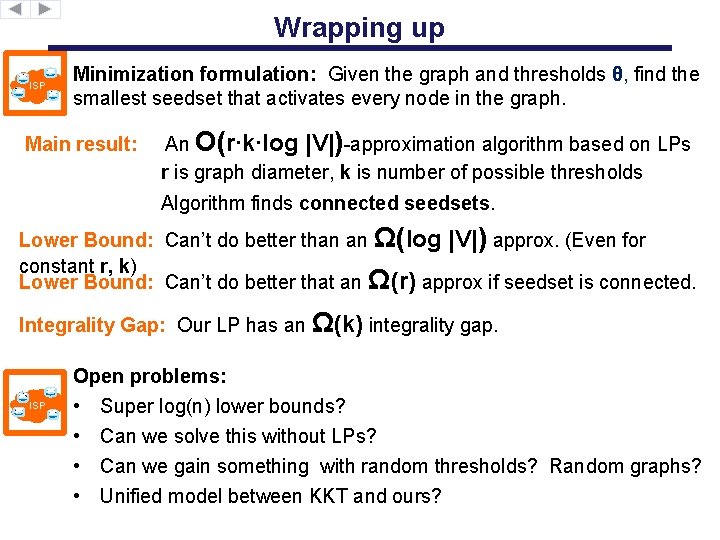
Wrapping up ISP Minimization formulation: Given the graph and thresholds θ, find the smallest seedset that activates every node in the graph. Main result: An O(r∙k∙log |V|)-approximation algorithm based on LPs r is graph diameter, k is number of possible thresholds Algorithm finds connected seedsets. Lower Bound: Can’t do better than an Ω(log |V|) approx. (Even for constant r, k) Lower Bound: Can’t do better that an Ω(r) approx if seedset is connected. Integrality Gap: Our LP has an Ω(k) integrality gap. ISP Open problems: • Super log(n) lower bounds? • Can we solve this without LPs? • Can we gain something with random thresholds? Random graphs? • Unified model between KKT and ours?

Thanks! ISP Full report: http: //arxiv. org/abs/1202. 2928 Princeton University
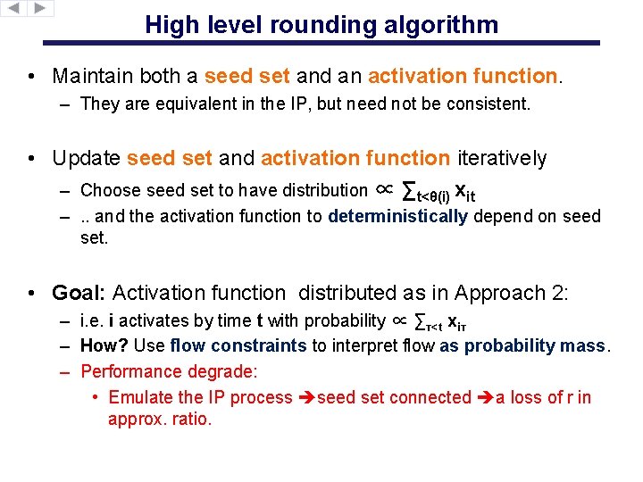
High level rounding algorithm • Maintain both a seed set and an activation function. – They are equivalent in the IP, but need not be consistent. • Update seed set and activation function iteratively – Choose seed set to have distribution ∝ ∑t<θ(i) xit –. . and the activation function to deterministically depend on seed set. • Goal: Activation function distributed as in Approach 2: – i. e. i activates by time t with probability ∝ ∑τ<t xiτ – How? Use flow constraints to interpret flow as probability mass. – Performance degrade: • Emulate the IP process seed set connected a loss of r in approx. ratio.
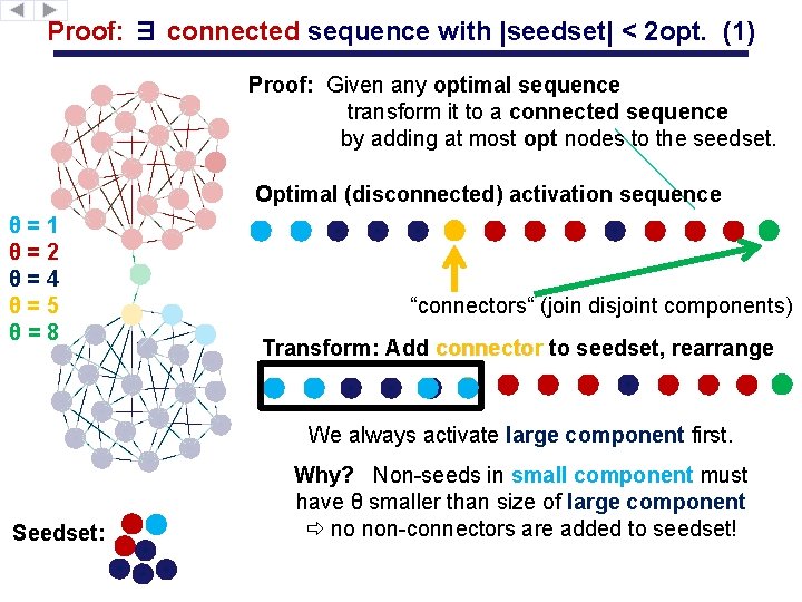
Proof: ∃ connected sequence with |seedset| < 2 opt. (1) Proof: Given any optimal sequence transform it to a connected sequence by adding at most opt nodes to the seedset. Optimal (disconnected) activation sequence θ=1 θ=2 θ=4 θ=5 θ=8 “connectors“ (join disjoint components) Transform: Add connector to seedset, rearrange We always activate large component first. Seedset: Why? Non-seeds in small component must have θ smaller than size of large component no non-connectors are added to seedset!
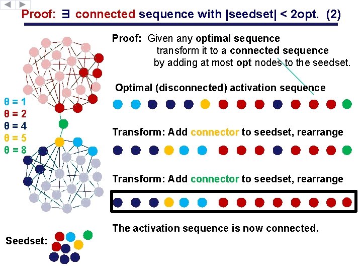
Proof: ∃ connected sequence with |seedset| < 2 opt. (2) Proof: Given any optimal sequence transform it to a connected sequence by adding at most opt nodes to the seedset. Optimal (disconnected) activation sequence θ=1 θ=2 θ=4 θ=5 θ=8 Transform: Add connector to seedset, rearrange The activation sequence is now connected. Seedset:
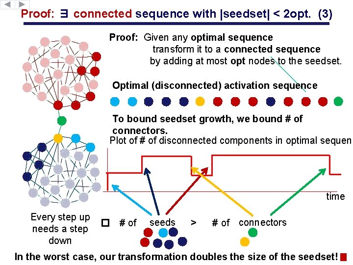
Proof: ∃ connected sequence with |seedset| < 2 opt. (3) Proof: Given any optimal sequence transform it to a connected sequence by adding at most opt nodes to the seedset. Optimal (disconnected) activation sequence To bound seedset growth, we bound # of connectors. Plot of # of disconnected components in optimal sequenc time Every step up needs a step down � # of seeds > # of connectors In the worst case, our transformation doubles the size of the seedset!

Part II: How do we round this? Iterative and adaptive rounding with both the seedset and sequence. We return connected seedsets instead of connected activation sequences. (�O(r)-approx instead of 2 -approx ) Princeton University
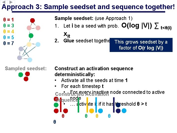
Approach 3: Sample seedset and sequence together! θ=1 θ=3 θ=4 θ=5 θ=7 Sampled seedset: Sample seedset: (use Approach 1) 1. Let i be a seed with prob. O(log xit |V|) ∑ t<θ(i) 2. Glue seedset together so it’sgrows connected This seedset by a factor of O(r log |V|) Construct an activation sequence deterministically: • Activate all the seeds at time 1 • For each timestep t • For every inactive node connected to active Constructed Activation node Sequence: • … activate it if it has threshold θ > t θ θ θ
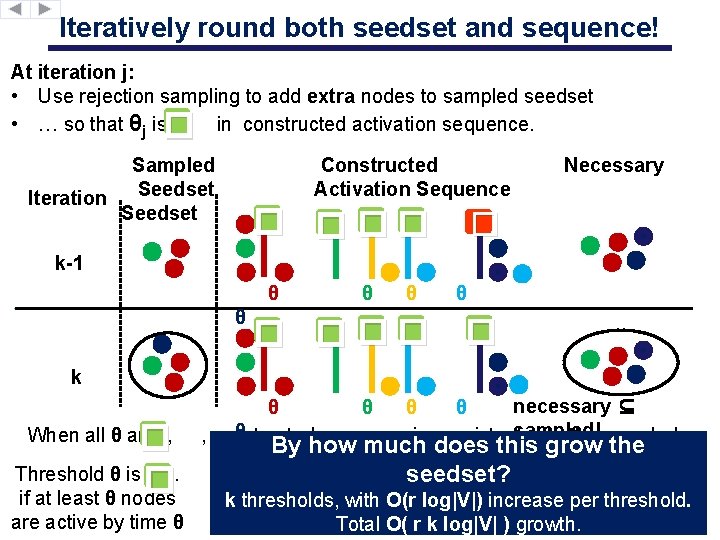
Iteratively round both seedset and sequence! At iteration j: • Use rejection sampling to add extra nodes to sampled seedset • … so that θj is. in constructed activation sequence. � Sampled Seedset Iteration Seedset Constructed Activation Sequence � ��� Necessary � k-1 θ θ � ��� θ � k � Threshold θ is �. if at least θ nodes When all θ are , are active by time θ necessary ⊆ θ θ θ , constructed sequence is consistentsampled! the sampled By how much does thiswith grow the seedset? k thresholds, with O(r log|V|) increase per threshold. Total O( r k log|V| ) growth.
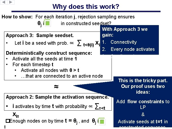
Why does this work? How to show: For each iteration j, rejection sampling ensures θj is in constructed seedset? With Approach 3 we gain: Approach 3: Sample seedset. � Let i be a seed with prob. ∝ ∑ t<θ(i) xit 1. Connectivity 2. Every node activates Deterministically construct sequence: 3. Small seedset • Activate all the seeds at time 1 • For each timestep t • Activate all nodes with θ > t • …that are connected to an active node This is the tricky part. Our proof uses two ideas: Approach 2: Sample the activation sequence. Add flow constraints to • i activates by time t with probability ∝ ∑τ<t LP & xiτ �Enough nodes on by time t = θj , and θj is Activate seeds at t=1 in constructed sequence. • ≈ �
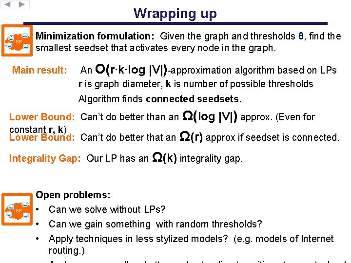
Wrapping up ISP Minimization formulation: Given the graph and thresholds θ, find the smallest seedset that activates every node in the graph. Main result: An O(r∙k∙log |V|)-approximation algorithm based on LPs r is graph diameter, k is number of possible thresholds Algorithm finds connected seedsets. Lower Bound: Can’t do better than an Ω(log |V|) approx. (Even for constant r, k) Lower Bound: Can’t do better that an Ω(r) approx if seedset is connected. Integrality Gap: Our LP has an Ω(k) integrality gap. ISP Open problems: • Can we solve without LPs? • Can we gain something with random thresholds? • Apply techniques in less stylized models? (e. g. models of Internet routing. )
Thanks! ISP To appear at SODA’ 13 http: //arxiv. org/abs/1202. 2928 Princeton University
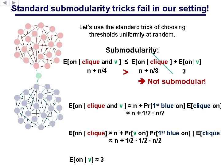
Standard submodularity tricks fail in our setting! Let’s use the standard trick of choosing thresholds uniformly at random. Submodularity: E[on | clique and v ] ≤ E[on | clique ] + E[on| v] n + n/4 n + n/8 3 > Not submodular! E[on | clique and v ] ≈ n + Pr[1 st blue on] E[clique on] ≈ n + 1/2 ∙ n/2 E[on | clique] ≈ n + Pr[v on] Pr[1 st blue on] ] E[clique ≈ n + 1/2 ∙ n/2 E[on | v] ≈ 3
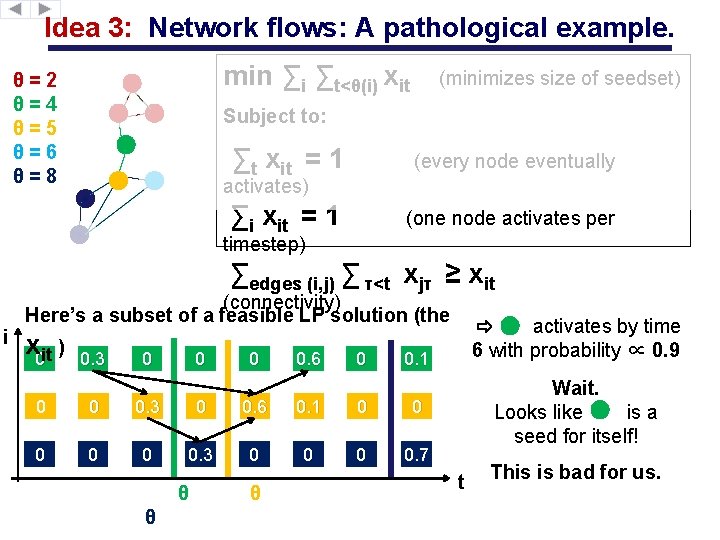
Idea 3: Network flows: A pathological example. min ∑i ∑t<θ(i) xit θ=2 θ=4 θ=5 θ=6 θ=8 (minimizes size of seedset) Subject to: ∑t xit = 1 (every node eventually ∑i xit = 1 (one node activates per activates) timestep) ∑edges (i, j) ∑ τ<t xjτ ≥ xit x 0 it ) 0. 3 0 0. 6 0 0. 1 0 0 0. 3 0 0. 6 0. 1 0 0 0. 3 0 0. 7 θ θ θ activates by time 6 with probability ∝ 0. 9 Wait. Looks like is a seed for itself! i (connectivity) Here’s a subset of a feasible LP solution (the t This is bad for us.
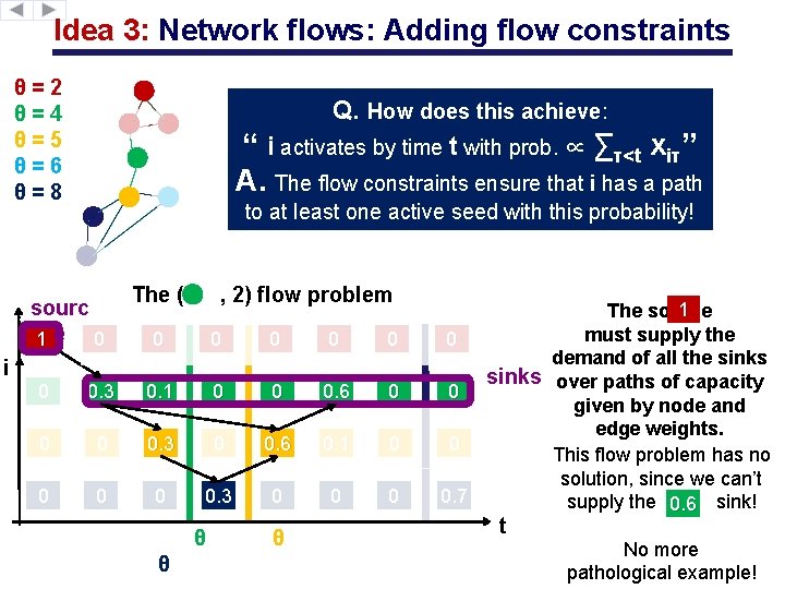
Idea 3: Network flows: Adding flow constraints θ=2 θ=4 θ=5 θ=6 θ=8 Q. How does this achieve: We add a few extra constraints to the LP activates abysource time tnode with prob. to∝ ∑τ<tat xtime 1)“ i. Constrain start iτ” 1 2) solution to ensure each (i, t) problem. A. Require The flowaconstraints thatflow i has a path to at least one active seed with this probability! sourc i e 1 0 The ( , 2) flow problem 0 0 0 i 0 0. 3 0. 1 0 0 0. 6 0 0. 3 0 0. 6 0. 1 0 0 0. 3 0 0 0 θ θ θ 1 The source must supply the 0 demand of all the sinks over paths of capacity 0 given by node and edge weights. 0 This flow problem has no solution, since we can’t 0. 7 supply the 0. 6 sink! t No more pathological example!
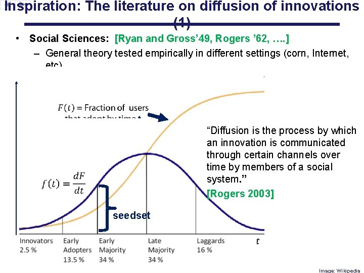
Inspiration: The literature on diffusion of innovations (1) • Social Sciences: [Ryan and Gross’ 49, Rogers ’ 62, …. ] – General theory tested empirically in different settings (corn, Internet, etc) “Diffusion is the process by which an innovation is communicated through certain channels over time by members of a social system. ” [Rogers 2003] seedset Image: Wikipedia
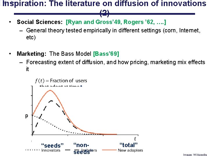
Inspiration: The literature on diffusion of innovations (2) • Social Sciences: [Ryan and Gross’ 49, Rogers ’ 62, …. ] – General theory tested empirically in different settings (corn, Internet, etc) • Marketing: The Bass Model [Bass’ 69] – Forecasting extent of diffusion, and how pricing, marketing mix effects it p “seeds” “nonseeds” “total” Image: Wikipedia
Inspiration: The literature on diffusion of innovations (3) • Social Sciences: [Ryan and Gross’ 49, Rogers ’ 62, …. ] – General theory tested empirically in different settings (corn, Internet, etc) • Marketing: The Bass Model [Bass’ 69] – Forecasting extent of diffusion, and how pricing, marketing mix effects it • Economics: “Network externalities” or “Network effects” [Katz Shapiro’ 85…] – Models to analyze markets, econometric validation, etc “The utility that a given user derives from the good depends upon the number of other users who are in the same “network” as he or she. ” [Katz & Shapiro 1985]
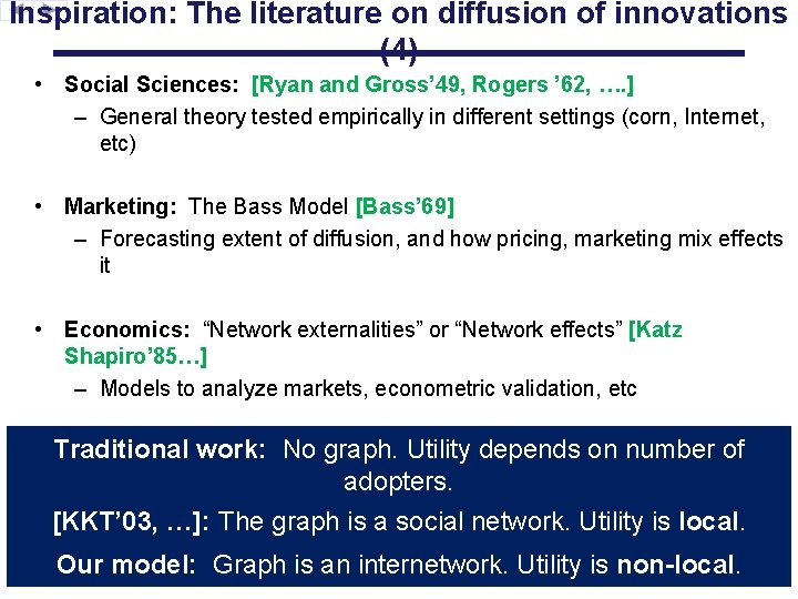
Inspiration: The literature on diffusion of innovations (4) • Social Sciences: [Ryan and Gross’ 49, Rogers ’ 62, …. ] – General theory tested empirically in different settings (corn, Internet, etc) • Marketing: The Bass Model [Bass’ 69] – Forecasting extent of diffusion, and how pricing, marketing mix effects it • Economics: “Network externalities” or “Network effects” [Katz Shapiro’ 85…] – Models to analyze markets, econometric validation, etc work: “Metcalfe’s No graph. Utility depends • Traditional Popular Science: Law” [Metcalfe 1995]on number of “The utility that aadopters. single user gets for being part of a network of n users scales as n. ” [KKT’ 03, …]: The graph is a social network. Utility is local. [Metcalfe, (inventor of Ethernet!), 1995] Our model: Graph is an internetwork. Utility is non-local.
Part I: From global to local. (via a 2 -approximation ) Princeton University
- Slides: 40