Diffractive Pupil Telescope for highprecision space astrometry and

Diffractive Pupil Telescope for high-precision space astrometry (and coronagraphy!) Olivier Guyon (Uof. A) Michael Shao (NASA JPL) Improvements to original concept, error budget, exoplanet science Stuart Shaklan (NASA JPL) Error budget, mission architecture Robert Woodruff (LMC) Optical design for wide field telescope compatible with coronagraphy Bijan Nemati (NASA JPL) Numerical simulations, modeling approach Mark Ammons (Uof. A) Lab demo design & operation Eduardo Bendek (Uof. A) Lab demo optical design & operation Marie Levine (NASA JPL) System engineering, mission architecture Joe Pitman (Expl. Sci. ) System engineering Tom Milster (Uof. A) Mask manufacturing, scaling of mask manufacturing to full scale PM Jim Burge (Uof. A) Mask manufacturing, scaling of mask manufacturing to full scale PM Neville Woolf (Uof. A) Exoplanet science, concept definition Roger Angel (Uof. A) Exoplanet science, concept definition Josh Eisner (Uof. A) Exoplanet and star formation/evolution science Ruslan Belikov (NASA Ames) Compatibility with coronagraphy Daniel Eisenstein (Uof. A) Extragalactic science enabled with wide field camera Ann Zabludoff (Uof. A) Extragalactic science with wide field camera Dennis Zaritsky (Uof. A) Extragalactic & galactic science with wide field camera Jay Daniel (L 3/Tinsley) Optics manufacturing

Principle: use background stars around coronagraph target as an astrometric reference With a 1. 4 -m telescope in the visible, 0. 25 sq deg offers sufficient photons from stars at the galactic pole to provide an astrometric reference at the <50 nano-arcsec after taking into account realistic efficiency, zodi light and pixel sampling. Why is imaging astrometry difficult ? (1) Light from different stars on the sky travels different paths → small bending of optics produces field distortions (2) The detector can move between observations (especially when using large mosaics) (3) Pixels are not perfect and their response changes with time + (4) Central star is much brighter than background stars

Optical Layout for simultaneous coronagraphy and astrometry The telescope is a conventional TMA, providing a high quality diffraction-limited PSF over a 0. 5 x 0. 5 deg field with no refractive corrector. The design shown here was made for a 1. 4 m telescope (PECO). Light is simultaneously collected by the coronagraph instrument (direct imaging and spectroscopy of exoplanet) and the wide field astrometric camera (detection and mass measurement of exoplanets) M 1 is covered with small dots M 1 Coronagraph instrument Central ~10” field M 2 wide field image for astrometry Intermediate focal plane M 3

Dots on primary mirror create a series of diffraction spikes used to calibrate astrometric distortions The center of the field is missing from the astrometric camera (central light is sent to coronagraph) Primary mirror is covered with small dots Dots create spikes in the wide field astrometric camera All astrometric distortions (due to change in optics shapes of M 2, M 3, and deformations of the focal plane array) are common to the spikes and the background stars. By referencing the background star positions to the spikes, the astrometric measurement is largely immune to large scale astrometric distortions. Instead of requiring ~pm level stability on the optics over yrs, the stability requirement on M 2, M 3 is now at the nm-level over approximately a day on the optics surfaces, which is within expected stability of a coronagraphic space telescope. (Note: the concept does not require stability of the primary mirror).

Precursors. . . “Long-focus photographic astrometry”, van de Kamp, 1951 “Astrometry and Photometry with Coronagraphs”, Sivaramakrishnan, Anand; Oppenheimer, Ben R. , 2006

Red points show the position of background stars at epoch #1 (first observation)

Blue points show the position of background stars at epoch #2 (second observation) The telescope is pointed on the central star, so the spikes have not moved between the 2 observations, but the position of the background stars has moved due to the astrometric motion of the central star (green vectors).

Due to astrometic distortions between the 2 observations, the actual positions measured (yellow) are different from the blue point. The error is larger than the signal induced by a planet, which makes the astrometric measurement impossible without distortion calibration.

The measured astrometric motion (blue vectors in previous slide) is the sum of the true astrometric signal (green vectors) and the astrometric distortion induced by change in optics and detector between the 2 observations. Direct comparison of the spike images between the 2 epochs is used to measure this distortion, which is then subtracted from the measurement to produce a calibrated astrometric measurement.

The calibration of astrometric distortions with the spikes is only accurate in the direction perpendicular to the spikes length. For a single background star, the measurement is made along this axis (1 -D measurement), as shown by the green vectors. The 2 -D measurement is obtained by combining all 1 -D measurements (large green vector).

Observation scheme The green vector is what should be measured A slow telescope roll is used to average out small scale distortions, which are due to non-uniformity in the pixel size, (spectral) response, and geometry Telescope roll angle coronagraph field star 1 star 2 Epoch #1 Epoch #2 Proper motion + Parallax + astrometric signal diffraction spikes

Science goals Primary science goal: Measure planet mass with 10% accuracy (1 -σ) for an Sun/Earth analog at 6 pc. This allows mass measurement of all potentially habitable planets (Earth-like & Super. Earths) imaged by PECO. SNR>5 detection at R=5 in less than 6 hrs along 20% of the planet orbit, assuming 45% system efficiency, and 1 zodi (no WF errors) Table extracted from PECO SRD (http: //caao. as. arizona. edu/PECO_SRD. pdf)

Simulated observations Planetary system characteristics Star Sun analog Distance 6 pc Location Ecliptic pole Orbit semi-major axis 1. 2 AU Planet mass 1 Earth mass Orbit excentricity 0. 2 Astrometric signal amplitude 0. 5 μas Orbit apparent semi-major axis 200 mas Observations Number of observations Coronagraph: planet position measurement accuracy in coronagraphic image Coronagraph: Inner Working Angle Astrometry: accuracy 32 (regularly spaced every 57 days) 2. 5 mas per axis (= 3. 6 mas in 2 D): corresponds to diffraction-limited measurement with 100 photon at 550 nm on PECO 130 mas (coronagraph cannot see planet inside IWA) Variable (to be matched to science requirements)

Combined solution derived from simultaneous coronagraphy and astrometry measurements Measurements Known variables: - Star location on the sky (effect of parallax is known except for star distance, aberration of light perfectly known) - observing epochs - Stellar mass (assumed to be known at the 5% accuracy level) - measurement noise levels for astrometry (~μas), coronagraphy planet position (few mas) and star mass (~5%) Astrometry: star position (nb of variables = 2 x #observations) Coronagraphy: planet position (nb of variables = 2 x #observations) Solution Maximum likelihood solution for 11 free parameters to be solved for: - star parallax (1 variable) - proper motion (2 variables) - star mass (1 variable) - planet mass (1 variable) - orbital parameters (6 variables)

Combined solution for simultaneous coronagraphy + astrometry Planet on a 1. 2 AU orbit (1. 3 yr period), e=0. 2 orbit orientation on sky: planet outside the coronagraph IWA for 17 out of the 32 observations. Coronagraph IWA (130 mas radius) Required single measurement astrometric accuracy = 0. 2 μas (1 sigma, 1 D)

Combined solution for simultaneous coronagraphy + astrometry is very accurate for orbital parameters measurement

Better estimate of orbital parameters -> better planet mass estimate This plot shows correlation between semi-major axis and planet mass in astrometry measurement smaller error in semi-major axis -> better mass estimate

Better estimate of stellar mass -> better planet mass estimate This plot shows correlation between stellar mass and planet mass in astrometry measurement direct measurement of stellar mass -> better planet mass estimate

Combined solution for simultaneous coronagraphy + astrometry Standard deviation Astrometry only Astrometry + coronagraphy 0. 037 μas 0. 035 μas x proper motion 0. 017 μas/yr 0. 012 μas/yr y proper motion 0. 020 μas/yr 0. 013 μas/yr Planet mass 0. 132 ME 0. 098 ME Semi-major axis 0. 0228 AU 0. 0052 AU orbital phase 0. 653 rad orbit inclination 0. 0968 rad sma projected PA on sky 0. 1110 rad 0. 0040 rad 0. 098 0. 0035 0. 648 rad 0. 0034 rad parallax orbit ellipticity PA of perihelion on orbit plane (w) stellar mass 0. 050 MSun ~10 x better estimate on orbital parameters Direct stellar mass measurement 0. 039 rad 0. 0065 rad 0. 013 MSun

Benefits of simultaneous coronagraphy + astrometry Solving for planet orbit and mass using the combined astrometry + coronagraphy measurements is scientifically very powerful: - Reduces confusion with multiple planets. Outer massive planets (curve in the astrometric measurement) will be seen by the coronagraph. - Astrometry will separate planets from exozodi clumps. - Astrometric knowledge allows to extract fainter planets from the images, especially close to IWA, where the coronagraph detections are marginal. - Mitigates the 1 yr period problem for astrometry

Value in simulations Telescope diameter (D) 44 mas 0. 03 sq deg (0. 1 deg radius) Rationale for flight instrument value Impact on astrometric accuracy Astrometric accuracy goes as D-2, thanks PECO sized, cost constrained to larger collecting area and smaller PSF size (assuming constant FOV) 1. 4 m Detector pixel size Field of view (FOV) Value for mission 0. 25 sq deg (0. 5 deg X 0. 5 deg) Nyquist at 600 nm Little impact as long as sampling is close to or finer than Nyquist low WF error across field, 1. 6 Gpix detector Astrometric accuracy goes as FOV-0. 5 Typical single observation duration for coronagraph Astrometric accuracy goes as t-0. 5 8% Keeps thoughput loss moderate in coronagraph Larger dot coverage allows observation of fainter sources. Flat field error after calibration, static (high spatial frequency) 1. 02% RMS, 6% peak Conservative estimate for modern detector after calibration Negligible effect on background PSF measurement (well averaged with roll) Flat field error, dynamic 1 e-4 RMS per pixel, uncorrelated spatially and temporally between observations 1 e-4 loss in sensitivity for each pixel over 48 hrs = 2% per year = 10% over 5 yrs Negligible effect on background PSF measurement, but significant effect on measurement of spikes locations 1. 0 rad (+/- 0. 5 rad) Manageable sunshielding 40 pm Wavefront measurement repeatability (optical element removed / reinserted) obtained when testing similar sized optics on ground 1. 5 nm WF error and PSD taken from Small impact on performance, as background PSFs are almost fixed similar existing optical between observations element Single measurement time Dot coverage on PM (area) Telescope roll 48 hr 1% Uncalibrated change in optics surface between observations for M 2 & M 3 Static optics surface errror (M 3 mirror) Astrometric accuracy, single measurement, single axis, m. V=3. 7, galactic pole 0. 58 μas 0. 20 μas 0. 2 μas is required to achieve science goals Larger telescope roll leads to better averaging of detector errors Larger change in optics surface reduces astrometric accuracy

Simulation description Simulation details available on: www. naoj. org/staff/guyon/ (60 slides describing next chart) Simulation assumes: • 1. 4 m telescope TMA (Woodruff design) • 1. 5 nm surface (3 nm WF) optics for M 2 and M 3, PSD provided by Tinsley • Circular field of view, 0. 2 deg diam (0. 03 sq deg) • Galactic pole observation (worst case scenario) • central star is m. V=3. 7 (faintest of the 7 PECO targets for which an Earth can be imaged in <6 hr, 14 th brightest target in the 20 high priority targets list) • 90% detector peak QE, 80% optical throughput (0. 963 for optics reflectivity x 0. 92 due to dots on PM) • Nyquist sampled detector at 0. 6 micron = 44 mas pixels • Telescope roll = 1 rad (larger angle = better averaging, but more difficult to maintain stability) • Single epoch observation = 2 day Distortions in the system are computed with 3 D raytracing (code written in C, agreement with Code V results from Woodruff has been checked) Images produced by Fourier transform, and then distorted according to geometrical optics. Image sizes are 16 k x 16 k.

Numerical simulation approach pupil mask with dots Monochromatic PSF Polychromatic PSF pupa psf 1 m psf 1 p Dyn ami c d i s to r ti o n s focal plane array x and y distortion change fpdistx, fpdisty mirrors M 2 and M 3 surface change psfpdx, psfpdy total x and y distortion change + variation in detector flat field response angular distortion change optics x and y distortion change distr x optdistx, optdisty binned angular distortion change fferror photon noise error due to zodiacal light and stellar flux x distx, disty raytracing distvarx, distvary psfpdr signal photon noise due to zodiacal background and stellar flux signal / - measured spikes image mpsf snrim square & bin + distrbin background star position measurement error (angular direction) distortion measurement SNR per pixel for a 1 pixel angular distortion PSF angular derivative PSF x derivative PSF y derivative binned square SNR per pixel for a 1 pixel angular distortion snr 2 bin SNR^2 -weighted binning binned angular distortion signalbin SNR-weighted binned angular convolution by anisoplanatism sized distortion measurement kernel quick look at residual distortion (useful for optimizing anisoplanatism kernel) roll averaged residual distortion error map in roll averaging residual astrometric angular direction distortion error map in astrerrordyn angular direction roll averaging resdist mdistrbin bilinear interpolation measured astrometric distortion map in angular direction mdistr ffsta distr_sta S ta ti c d i s to r ti o n s focal plane array x and y distortion + fpdistx_sta, fpdisty_sta mirrors M 2 and M 3 surface errors total x and y distortion distx_sta, disty_sta raytracing optics x and y distortion optdistx_sta, optdisty_sta background stars position measurement errors between 2 epochs (1 -D angular coordinate) optimal weighting of all 1 -D measurements 2 -D astrometric measurement Sum of two or more images x static angular distortion - detector flat field error Difference between two images Product of two images (pixel by pixel) Image name (used through this document) Operation performed on images or data

good detector calibration stable optical system and focal plane array Detector saturation poor detector calibration unstable optical system and focal plane array shorter detector readout shorter observation time finite detector sampling, polychromatic PSF zodi background longer observation time accuracy floor due to distortions & detector limits 1. 4 m telescope 0. 1 deg field radius (0. 03 sq deg) galactic pole 2 day observation

Performance as a function of star brightness (FOV = 0. 03 sq deg) Diffraction spikes become too faint to accurately calibrate astrometric distortions Performance limited by systematics and brightness, number of background stars

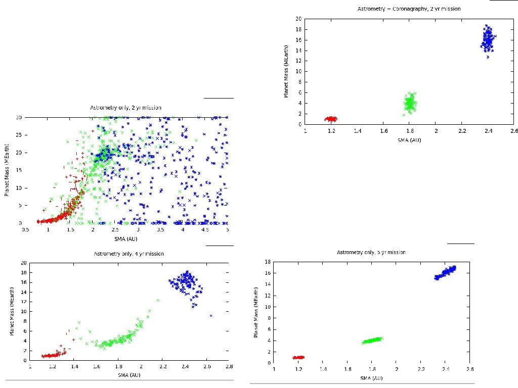
Astrometry + coronagraphy can precisely measure mass and orbital parameters of multiple planets systems Astrometry+Coronagraphy, Coronagraphy only : 1 observation every 2 month Astrometry only: 1 observation per month

Mass can be constrained quickly → firm identification of Earth-like planets within 1 to 2 yrs

8 % area coverage on PM m. V = 3. 7 target Galactic pole observation 2 day per observation Larger telescope diameter : - more light in spikes (D 2), finer spikes (1/D) → spike calibration accuracy goes as D-2 - more light in background stars (D 2), and smaller PSF (1/D) → position measurement goes as D-2 Astrometric accuracy goes as D-2 FOV-0. 5 Number of pixels goes as D-2 FOV At fixed number of pixels, larger D is better But: mean surface brightness of spikes gets fainter as FOV increases FOV = 0. 03 sq deg D = 1. 4 m D = 2. 0 m D = 3. 0 m D = 4. 0 m FOV = 0. 1 sq deg FOV = 0. 25 sq deg FOV = 0. 5 sq deg FOV = 1. 0 sq deg 0. 58 μas 0. 31 μas 0. 20 μas 0. 14 μas 0. 11 μas 0. 28 μas 0. 15 μas 0. 10 μas 0. 07 μas 0. 05 μas 0. 13 μas 0. 067 μas 0. 044 μas 0. 030 μas 0. 024 μas 0. 071 μas 0. 038 μas 0. 025 μas 0. 017 μas 0. 013 μas D = 4. 0 m, FOV = 0. 1 sq deg → 0. 2 uas in <2 hr

Conclusions For more info: http: //www. naoj. org/staff/guyon/04 research. web/30 astrometry. web/content. html Wide field imaging, coronagraphy and astrometry could be done on the same Telescope, simultaneously Simultaneous astrometry + coronagraphy is extremely powerful – Improved detection – Mass measurement On-sky demonstration and science considered Lab demo has started at U of Arizona will be used to validate error budget and data reduction