Differential gene expression analysis DESeq 2 and edge

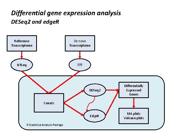
Differential gene expression analysis DESeq 2 and edge. R Reference Transcriptome De novo Transcriptome HTSeq ? ? ? DESeq 2 Differentially Expressed Genes Edge. R MA plots Volcano plots Counts R Statistical Analysis Package

Differential gene expression analysis The R Project • What is R? ? ? ◦ https: //www. r-project. org/ ◦ https: //cran. r-project. org/web/packages/ • How to run R ◦ Unix command line ◦ Rstudio – plots are a little more convenient ◦ R GUI – slightly less convenient for plots and help • On PC, run as administrator ◦ makes installing packages easier ◦ installation of base package takes a few minutes with fast internet ◦ update all/some/none? [a/s/n]: answer a

Rstudio on Scholar Add to. bash_profile if [[ -n $RSTUDIO_MULTI_SESSION ]]; then export RSTUDIO_SERVER=1 module purge module load gcc/5. 2. 0 fi • log out of scholar and log back in

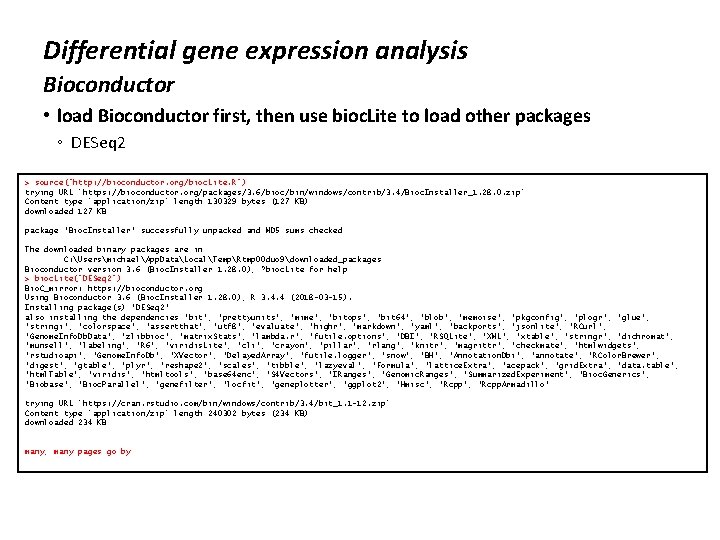
Differential gene expression analysis Bioconductor • load Bioconductor first, then use bioc. Lite to load other packages ◦ DESeq 2 > source("http: //bioconductor. org/bioc. Lite. R") trying URL 'https: //bioconductor. org/packages/3. 6/bioc/bin/windows/contrib/3. 4/Bioc. Installer_1. 28. 0. zip' Content type 'application/zip' length 130329 bytes (127 KB) downloaded 127 KB package ‘Bioc. Installer’ successfully unpacked and MD 5 sums checked The downloaded binary packages are in C: UsersmichaelApp. DataLocalTempRtmp 0 Oduo 9downloaded_packages Bioconductor version 3. 6 (Bioc. Installer 1. 28. 0), ? bioc. Lite for help > bioc. Lite("DESeq 2") Bio. C_mirror: https: //bioconductor. org Using Bioconductor 3. 6 (Bioc. Installer 1. 28. 0), R 3. 4. 4 (2018 -03 -15). Installing package(s) ‘DESeq 2’ also installing the dependencies ‘bit’, ‘prettyunits’, ‘mime’, ‘bitops’, ‘bit 64’, ‘blob’, ‘memoise’, ‘pkgconfig’, ‘plogr’, ‘glue’, ‘stringi’, ‘colorspace’, ‘assertthat’, ‘utf 8’, ‘evaluate’, ‘highr’, ‘markdown’, ‘yaml’, ‘backports’, ‘jsonlite’, ‘RCurl’, ‘Genome. Info. Db. Data’, ‘zlibbioc’, ‘matrix. Stats’, ‘lambda. r’, ‘futile. options’, ‘DBI’, ‘RSQLite’, ‘XML’, ‘xtable’, ‘stringr’, ‘dichromat’, ‘munsell’, ‘labeling’, ‘R 6’, ‘viridis. Lite’, ‘cli’, ‘crayon’, ‘pillar’, ‘rlang’, ‘knitr’, ‘magrittr’, ‘checkmate’, ‘htmlwidgets’, ‘rstudioapi’, ‘Genome. Info. Db’, ‘XVector’, ‘Delayed. Array’, ‘futile. logger’, ‘snow’, ‘BH’, ‘Annotation. Dbi’, ‘annotate’, ‘RColor. Brewer’, ‘digest’, ‘gtable’, ‘plyr’, ‘reshape 2’, ‘scales’, ‘tibble’, ‘lazyeval’, ‘Formula’, ‘lattice. Extra’, ‘acepack’, ‘grid. Extra’, ‘data. table’, ‘html. Table’, ‘viridis’, ‘htmltools’, ‘base 64 enc’, ‘S 4 Vectors’, ‘IRanges’, ‘Genomic. Ranges’, ‘Summarized. Experiment’, ‘Bioc. Generics’, ‘Biobase’, ‘Bioc. Parallel’, ‘genefilter’, ‘locfit’, ‘geneplotter’, ‘ggplot 2’, ‘Hmisc’, ‘Rcpp. Armadillo’ trying URL 'https: //cran. rstudio. com/bin/windows/contrib/3. 4/bit_1. 1 -12. zip' Content type 'application/zip' length 240302 bytes (234 KB) downloaded 234 KB many, many pages go by

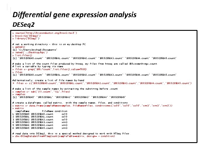
Differential gene expression analysis DESeq 2 > source("http: //bioconductor. org/bioc. Lite. R") > bioc. Lite("DESeq 2") > library("DESeq 2" ) # set a working directory – this is on my desktop PC > getwd() [1] "C: /Users/michael/Documents" > setwd('. . /Desktop/hpc') > list. files() [1] "SRR 5295840. count" "SRR 5295841. count" "SRR 5295842. count" "SRR 5295843. count“ "SRR 5295844. count" "SRR 5295845. count" # make a list of the count files produced by htseq, my files from htseq are called SRR<something>. count # list a variable by typing its name > files <- grep("SRR. *count", list. files(), value=TRUE) > files [1] "SRR 5295840. count" "SRR 5295841. count" "SRR 5295842. count" "SRR 5295843. count“ "SRR 5295844. count" "SRR 5295845. count" #alternatively, create a list of file names by hand Ø files <- c("SRR 5295840. count", "SRR 5295841. count", "SRR 5295842. count", "SRR 5295843. count", "SRR 5295844. count", "SRR 5295845. count") # make a list of the sample names by extracting the substring before. count > samples <- sub("(*). count", "\1", files) > samples [1] "SRR 5295840" "SRR 5295841" "SRR 5295842" "SRR 5295843" "SRR 5295844“ "SRR 5295845" # create a dataframe, called matrix, with the sample names, files, and conditions > matrix <- data. frame(sample. Name=samples, file. Name=files, condition=c("col 0", "xrn 3", "xrn 3")) > matrix sample. Name file. Name condition 1 SRR 5295840. count col 0 2 SRR 5295841. count col 0 3 SRR 5295842. count col 0 4 SRR 5295843. count xrn 3 5 SRR 5295844. count xrn 3 6 SRR 5295845. count xrn 3 # read data into DESeq 2, this is a special method designed to work with HTSeq files > ds<-DESeq. Data. Set. From. HTSeq. Count(sample. Table=matrix, design= ~ condition)

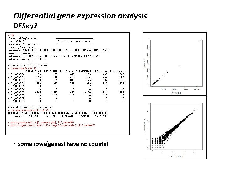
Differential gene expression analysis DESeq 2 > ds class: DESeq. Data. Set dim: 5537 6 5537 rows 6 columns metadata(1): version assays(1): counts rownames(5537): XLOC_000001 XLOC_000002. . . XLOC_005536 XLOC_005537 row. Data names(0): colnames(6): SRR 5295840 SRR 5295841. . . SRR 5295844 SRR 5295845 col. Data names(1): condition #look at the first 10 rows > counts(ds[1: 10, ]) SRR 5295840 SRR 5295841 SRR 5295842 SRR 5295843 SRR 5295844 SRR 5295845 XLOC_000001 159 168 162 193 228 XLOC_000002 139 135 121 144 136 150 XLOC_000003 88 86 100 74 94 89 XLOC_000004 280 367 359 353 527 572 XLOC_000005 0 0 0 2 0 0 XLOC_000006 0 0 0 XLOC_000007 1265 1557 1650 1130 1882 1999 XLOC_000008 0 0 0 XLOC_000009 0 1 1 0 0 0 XLOC_000010 0 0 0 # total counts in each sample > col. Sums(counts(ds[, 1: 6])) SRR 5295840 SRR 5295841 SRR 5295842 SRR 5295843 SRR 5295844 SRR 5295845 1167699 1396648 1415193 1097648 1749632 1756563 > plot(counts(ds[, 1]), counts(ds[, 2]), pch=20) > plot(log 10(counts(ds[, 1])), log 10(counts(ds[, 2])), pch=20) • some rows(genes) have no counts!

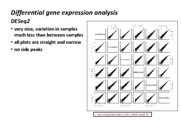
Differential gene expression analysis DESeq 2 • very nice, variation in samples much less than between samples • all plots are straight and narrow • no side peaks > pairs(log(counts(ds[, 1: 6])), ch=20, cex=0. 5)

Differential gene expression analysis DESeq 2 • scatterplot with transparency > plot(log(counts(ds[, 1])), log(counts(ds[, 4])), pch=20, col=rgb(1, 0, 0, 0. 05))

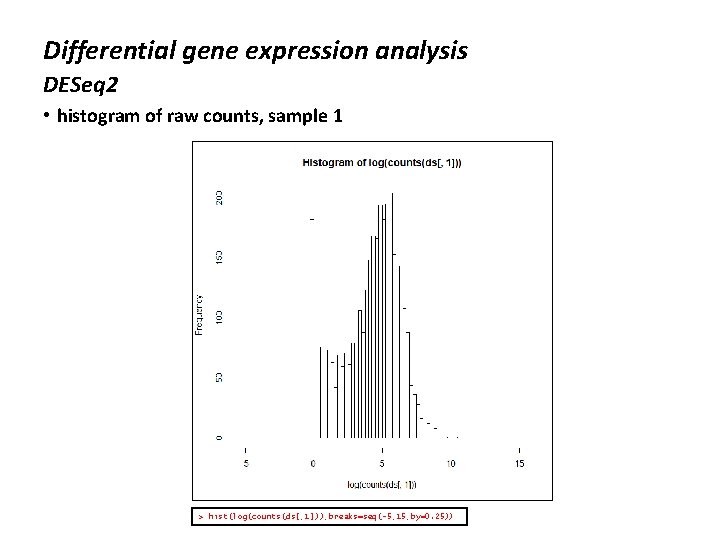
Differential gene expression analysis DESeq 2 • histogram of raw counts, sample 1 > hist(log(counts(ds[, 1])), breaks=seq(-5, 15, by=0. 25))

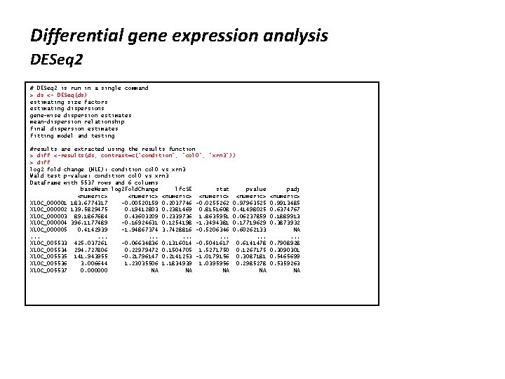
Differential gene expression analysis DESeq 2 # DESeq 2 is run in a single command > ds <- DESeq(ds) estimating size factors estimating dispersions gene-wise dispersion estimates mean-dispersion relationship final dispersion estimates fitting model and testing #results are extracted using the results function > diff <-results(ds, contrast=c("condition", "col 0", "xrn 3")) > diff log 2 fold change (MLE): condition col 0 vs xrn 3 Wald test p-value: condition col 0 vs xrn 3 Data. Frame with 5537 rows and 6 columns base. Mean log 2 Fold. Change lfc. SE stat pvalue <numeric> <numeric> XLOC_000001 183. 6774317 -0. 00520159 0. 2037746 -0. 0255262 0. 97963525 XLOC_000002 139. 5829475 0. 19412803 0. 2381469 0. 8151608 0. 41498025 XLOC_000003 89. 1867684 0. 43603209 0. 2339736 1. 8635951 0. 06237859 XLOC_000004 396. 1177489 -0. 16924631 0. 1254198 -1. 3494381 0. 17719629 XLOC_000005 0. 4142939 -1. 94867374 3. 7428816 -0. 5206346 0. 60262133. . . . XLOC_005533 425. 037261 -0. 06634836 0. 1316014 -0. 5041617 0. 6141478 XLOC_005534 294. 727806 0. 22979472 0. 1504705 1. 5271750 0. 1267175 XLOC_005535 141. 943955 -0. 21796147 0. 2141253 -1. 0179156 0. 3087181 XLOC_005536 3. 006644 1. 23035506 1. 1834939 1. 0395956 0. 2985278 XLOC_005537 0. 000000 NA NA padj <numeric> 0. 9913485 0. 6374767 0. 1889913 0. 3873932 NA. . . 0. 7908928 0. 3090301 0. 5465699 0. 5359263 NA

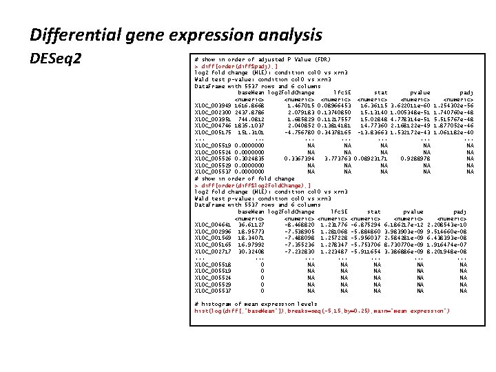
Differential gene expression analysis DESeq 2 # show in order of adjusted P Value (FDR) > diff[order(diff$padj), ] log 2 fold change (MLE): condition col 0 vs xrn 3 Wald test p-value: condition col 0 vs xrn 3 Data. Frame with 5537 rows and 6 columns base. Mean log 2 Fold. Change lfc. SE stat pvalue padj <numeric> <numeric> XLOC_003949 1616. 8668 1. 467015 0. 08966453 16. 36115 3. 622011 e-60 1. 254302 e-56 XLOC_002300 2437. 8786 2. 079183 0. 13740850 15. 13140 1. 005348 e-51 1. 740760 e-48 XLOC_003951 744. 0812 1. 685829 0. 11217557 15. 02848 4. 778314 e-51 5. 515767 e-48 XLOC_004746 1835. 1037 2. 040852 0. 13814181 14. 77360 2. 168122 e-49 1. 877052 e-46 XLOC_005175 151. 3101 -4. 756780 0. 34378165 -13. 83663 1. 532172 e-43 1. 061182 e-40. . . . . XLOC_005519 0. 0000000 NA NA NA XLOC_005524 0. 0000000 NA NA NA XLOC_005526 0. 3024835 0. 3367394 3. 773763 0. 08923171 0. 9288978 NA XLOC_005529 0. 0000000 NA NA NA XLOC_005537 0. 0000000 NA NA NA # show in order of fold change > diff[order(diff$log 2 Fold. Change), ] log 2 fold change (MLE): condition col 0 vs xrn 3 Wald test p-value: condition col 0 vs xrn 3 Data. Frame with 5537 rows and 6 columns base. Mean log 2 Fold. Change lfc. SE stat pvalue padj <numeric> <numeric> XLOC_004641 36. 61127 -8. 468820 1. 231776 -6. 875294 6. 186217 e-12 2. 208543 e-10 XLOC_002996 18. 95773 -7. 538905 1. 281068 -5. 884860 3. 983903 e-09 9. 514660 e-08 XLOC_001569 18. 34071 -7. 488098 1. 257228 -5. 956037 2. 584281 e-09 6. 438393 e-08 XLOC_005165 16. 97992 -7. 355236 1. 278347 -5. 753706 8. 730770 e-09 1. 916474 e-07 XLOC_002717 30. 32408 -7. 232830 1. 223487 -5. 911654 3. 386886 e-09 8. 201948 e-08. . . . . XLOC_005518 0 NA NA NA XLOC_005519 0 NA NA NA XLOC_005524 0 NA NA NA XLOC_005529 0 NA NA NA XLOC_005537 0 NA NA NA # histogram of mean expression levels hist(log(diff[, "base. Mean"]), breaks=seq(-5, 15, by=0. 25), main=“mean expression")

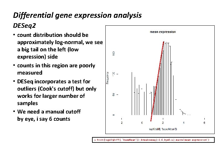
Differential gene expression analysis DESeq 2 • count distribution should be approximately log-normal, we see a big tail on the left (low expression) side • counts in this region are poorly measured • DESeq incorporates a test for outliers (Cook's cutoff) but only works for larger number of samples • We need a manual cutoff by eye, i say 6 counts > hist(log 10(diff[, "base. Mean"]), breaks=seq(-2, 6, by=0. 1), main="mean expression")

DESeq 2 • The idea of independent filtering is to filter out those tests from the procedure that have no, or little chance of showing significant evidence, without even looking at their test statistic. • Typically, this results in increased detection power at the same experiment-wide type I error (false discovery rate). • A good choice for a filtering criterion is one that ◦ is statistically independent from the test statistic under the null hypothesis, ◦ is correlated with the test statistic under the alternative, and ◦ does notably change the dependence structure – if any – between the test statistics of nulls and alternatives. • Filtering by total counts generally meets these criteria

DESeq 2 • manual cutoff > dds = ds[row. Sums(counts(ds[, 1: 6]))>40, ] > hist(log(counts(dds[, 1])), breaks=seq(-5, 15, by=0. 25)) > dds class: DESeq. Data. Set dim: 2862 6 metadata(1): version assays(3): counts mu cooks rownames(2862): XLOC_000001 XLOC_000002. . . XLOC_005534 XLOC_005535 row. Data names(21): base. Mean base. Var. . . deviance max. Cooks colnames(6): SRR 5295840 SRR 5295841. . . SRR 5295844 SRR 5295845 col. Data names(2): condition size. Factor • rerun DESeq on reduced set ◦ better able to see differences ◦ fewer spurious results

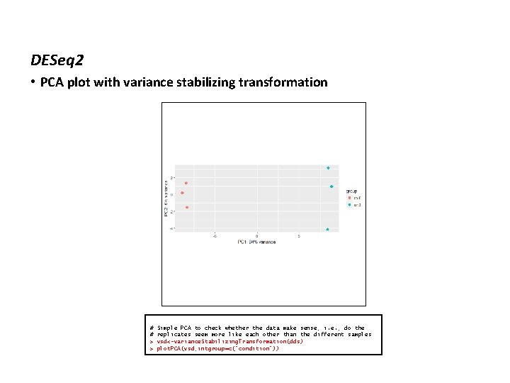
DESeq 2 • PCA plot with variance stabilizing transformation # # > > Simple PCA to check whether the data make sense, i. e. , do the replicates seem more like each other than the different samples vsd<-variance. Stabilizing. Transformation(dds) plot. PCA(vsd, intgroup=c("condition"))

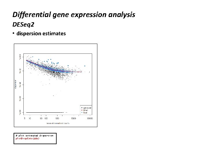
Differential gene expression analysis DESeq 2 • dispersion estimates # plot estimated dispersion plot. Disp. Ests(dds)

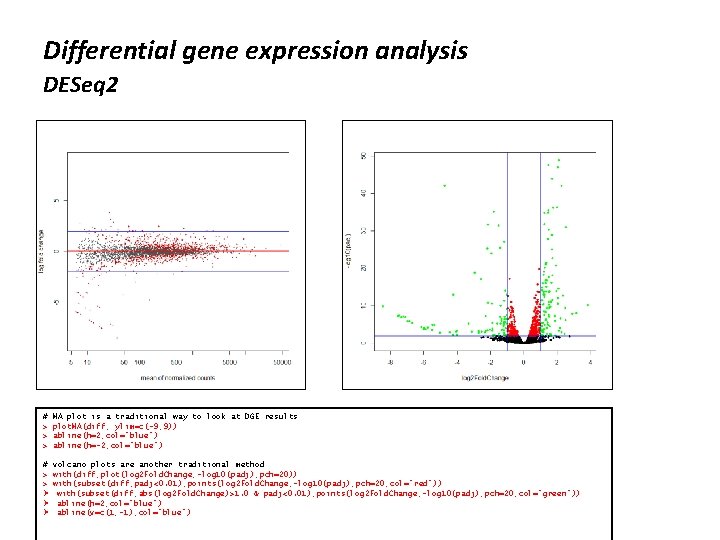
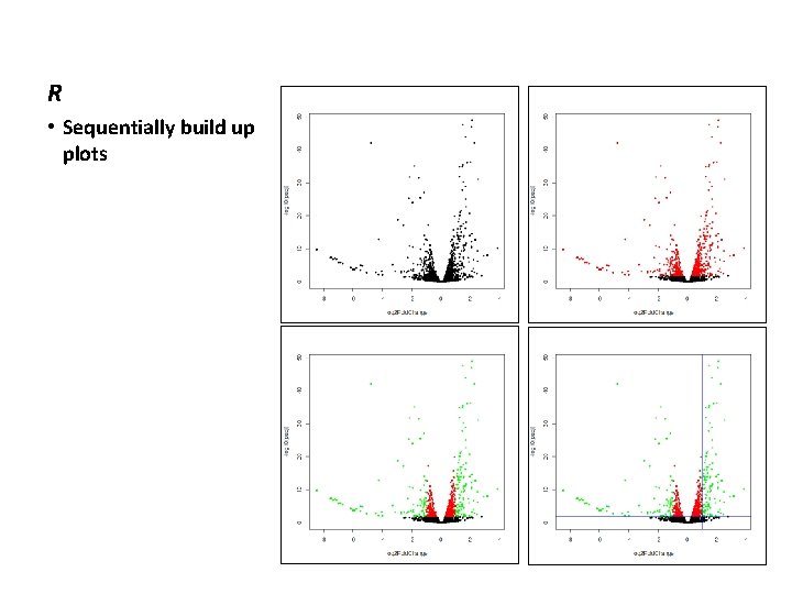
Differential gene expression analysis DESeq 2 # > > > MA plot is a traditional way to look at DGE results plot. MA(diff, ylim=c(-9, 9)) abline(h=2, col="blue") abline(h=-2, col="blue") # volcano plots are another traditional method > with(diff, plot(log 2 Fold. Change, -log 10(padj), pch=20)) > with(subset(diff, padj<0. 01), points(log 2 Fold. Change, -log 10(padj), pch=20, col="red")) Ø with(subset(diff, abs(log 2 Fold. Change)>1. 0 & padj<0. 01), points(log 2 Fold. Change, -log 10(padj), pch=20, col="green")) Ø abline(h=2, col="blue") Ø abline(v=c(1, -1), col="blue")

R • Sequentially build up plots

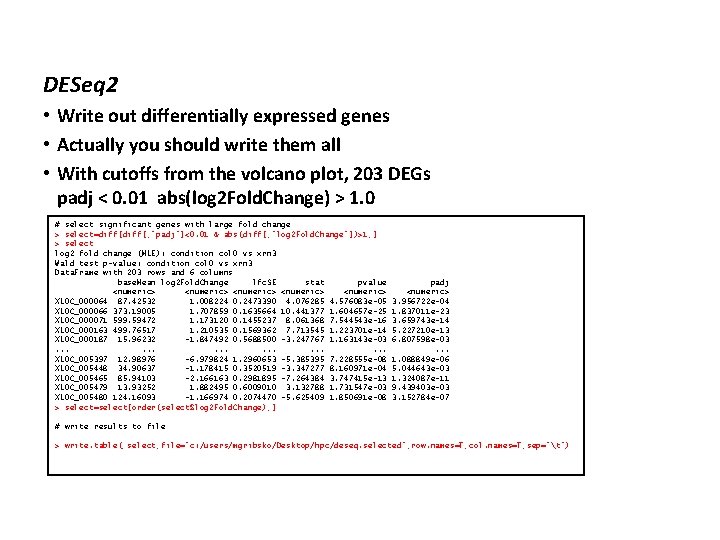
DESeq 2 • Write out differentially expressed genes • Actually you should write them all • With cutoffs from the volcano plot, 203 DEGs padj < 0. 01 abs(log 2 Fold. Change) > 1. 0 # select significant genes with large fold change > select=diff[, "padj"]<0. 01 & abs(diff[, "log 2 Fold. Change"])>1, ] > select log 2 fold change (MLE): condition col 0 vs xrn 3 Wald test p-value: condition col 0 vs xrn 3 Data. Frame with 203 rows and 6 columns base. Mean log 2 Fold. Change lfc. SE stat pvalue <numeric> <numeric> XLOC_000064 87. 42532 1. 008224 0. 2473390 4. 076285 4. 576083 e-05 XLOC_000066 373. 19005 1. 707859 0. 1635664 10. 441377 1. 604657 e-25 XLOC_000071 599. 59472 1. 173120 0. 1455237 8. 061368 7. 544543 e-16 XLOC_000163 499. 76517 1. 210535 0. 1569362 7. 713545 1. 223701 e-14 XLOC_000187 15. 96232 -1. 847492 0. 5688500 -3. 247767 1. 163143 e-03. . . . XLOC_005397 12. 98976 -6. 979824 1. 2960653 -5. 385395 7. 228555 e-08 XLOC_005448 34. 90637 -1. 178415 0. 3520519 -3. 347277 8. 160971 e-04 XLOC_005465 85. 94103 -2. 166163 0. 2981895 -7. 264384 3. 747415 e-13 XLOC_005479 13. 93252 1. 882495 0. 6009010 3. 132788 1. 731547 e-03 XLOC_005480 124. 16093 -1. 166974 0. 2074470 -5. 625409 1. 850691 e-08 > select=select[order(select$log 2 Fold. Change), ] padj <numeric> 3. 956722 e-04 1. 837011 e-23 3. 659743 e-14 5. 227210 e-13 6. 807598 e-03. . . 1. 088849 e-06 5. 044643 e-03 1. 324087 e-11 9. 439403 e-03 3. 152784 e-07 # write results to file > write. table( select, file="c: /users/mgribsko/Desktop/hpc/deseq. selected", row. names=T, col. names=T, sep="t")