Differential Equations MTH 242 Lecture 13 Dr Manshoor

Differential Equations MTH 242 Lecture # 13 Dr. Manshoor Ahmed

Summary (Recall) • Differential Operator, which is a linear operator. • Differential equation in linear operator form. • Auxiliary equation in terms of differential operator form. • Annihilator operators of different functions. • Solution non-homogeneous equation with annihilator operator.

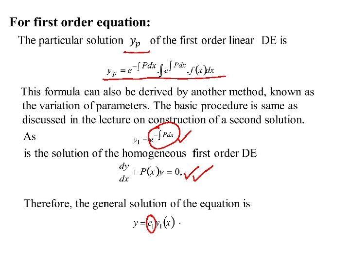
Method of variation of parameters

So that we obtain This is a variable separable equation. Thus, Integration gives As . Therefore, or .

Method for Second Order Equation: We consider the second order linear non-homogeneous DE Divide by , to get equation in the standard form , where are continuous on some interval I. Consider the associated homogeneous DE, .

Complementary function: Complementary function is So that Particular Integral For finding a particular solution , we replace the parameters and in the complementary function with the unknown variables and . So that the assumed particular integral is

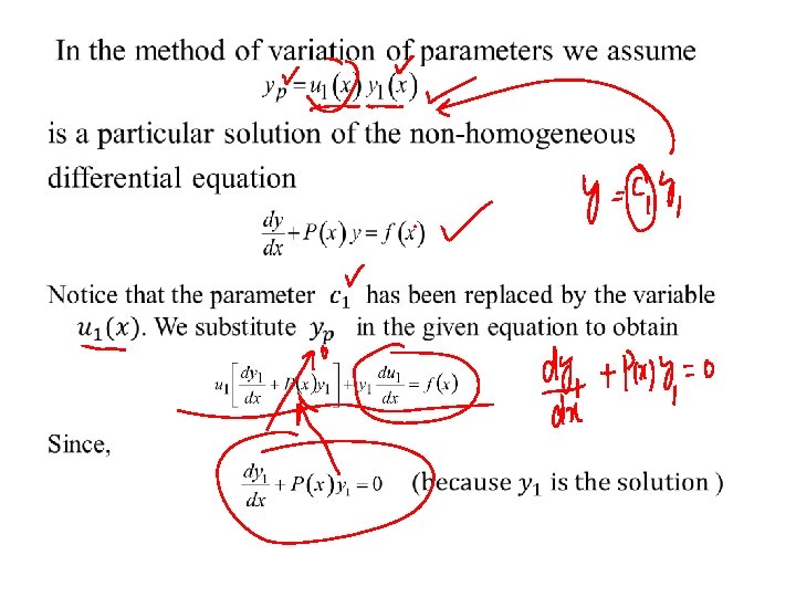
Since we seek to determine two unknown functions and , we need two equations involving these unknowns. One of these two equations results from substituting the assumed in the given differential equation. We impose the other equation to simplify the first derivative and thereby the 2 nd derivative of To avoid 2 nd derivatives of and , we impose the condition Then, So that Therefore,

Substituting in the given non-homogeneous differential equation yields or Now making use of the relations we get, Hence and must be functions that satisfy the equations By using the Cramer’s rule, the solution of this set of equations is given by

where and denote the following determinants The determinant can be identified as the Wronskian of the solutions . Since the solutions are linearly independent on I. Therefore Now integrating the expressions for we obtain the value of and , hence the particular solution of the non-homogeneous linear DE. Summary of the Method To solve the second order non-homogeneous linear DE using the variation of parameters, we need to perform the following steps:

Step 1 We find the complementary function by solving the associated homogeneous differential equation Step 2 If the complementary function of the equation is given by then are two linearly independent solutions of the homogeneous differential equation. Computing Wronskian. Step 3 By dividing with , we transform the given non-homogeneous equation into the standard form and we identify the function f(x).

Step 4 We now construct the determinants given by Step 5 Next we determine the derivatives of the unknown variables through the relations Step 6 Integrate the derivatives to find the unknown variables . So that Step 7 Write a particular solution of the given non-homogeneous equation as

Step 8 The general solution of the differential equation is then given by Constants of Integration We don’t need to introduce the constants of integration, when computing the indefinite integrals in step 6 to find the unknown functions of . For, if we do introduce these constants, then So that the general solution of the given non-homogeneous differential equation is or

If we replace with and with , we obtain This does not provide anything new and is similar to the general solution found in step 8, namely Example 1 Solve Solution: Step 1 To find the complementary function Put

Then the auxiliary equation is Repeated real roots of the auxiliary equation Step 2 By the inspection of the complementary function , we make the identification Therefore

Step 3 The given differential equation is Since this equation is already in the standard form Therefore, we identify the function as Step 4 We now construct the determinants

Step 5 We determine the derivatives of the functions in this step Step 6 Integrating the last two expressions, we obtain Remember! We don’t have to add the constants of integration. Step 7 Therefore, a particular solution of then given differential equation is

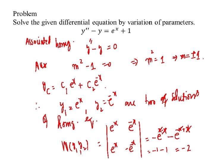
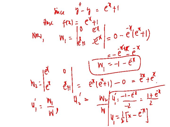
or Step 8 Hence, the general solution of the given differential equation is Example 2 Solve Solution: Step 1 To find the complementary function we solve the associated homogeneous differential equation The auxiliary equation is

Roots of the auxiliary equation are complex. Therefore, the complementary function is Step 2 From the complementary function, we identify as two linearly independent solutions of the associated homogeneous equation. Therefore Step 3 By dividing with , we put the given equation in the following standard form So that we identify the function as

Step 4 We now construct the determinants Step 5 Therefore, the derivatives are given by Step 6 Integrating the last two equations w. r. t , we obtain Here, no constants of integration are used.

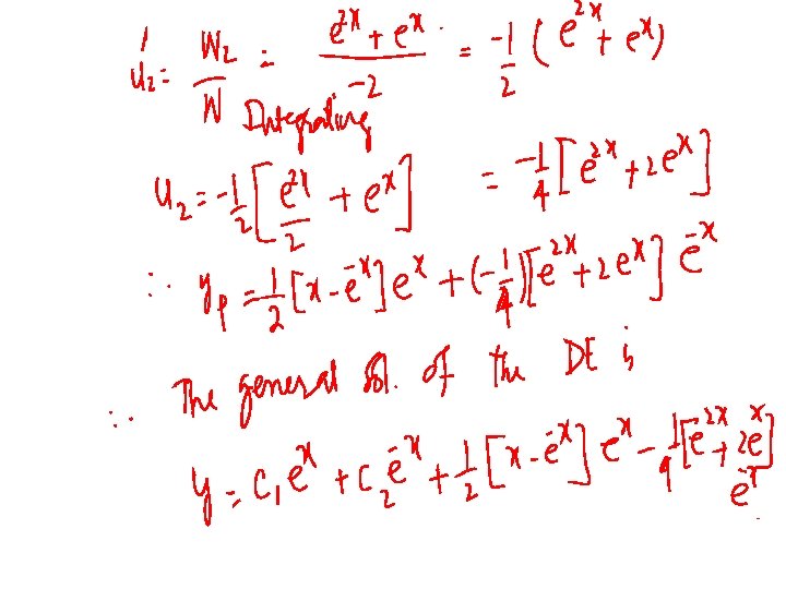
Step 7 The particular solution of the non-homogeneous equation is Step 8 Hence, the general solution of the given differential equation is Example 3 Solve Solution: Step 1 For the complementary function consider the associated homogeneous equation To solve this equation we put

Then the auxiliary equation is: The roots of the auxiliary equation are real and distinct. Therefore, the complementary function is Step 2 From the complementary function we find The functions are two linearly independent solutions of the homogeneous equation. The Wronskian of these solutions is Step 3 The given equation is already in the standard form

Here Step 4 We now form the determinants Step 5 Therefore, the derivatives of the unknown functions and are given by Step 6 We integrate these two equations to find the unknown functions

The integrals defining cannot be expressed in terms of the elementary functions and it is customary to write such integral as: Step 7 A particular solution of the non-homogeneous equations is Step 8 Hence, the general solution of the given differential equation is

For practice solve the problems from Exercise 4. 6 of your text book

Summary • Motivation for the method of variation of parameters. • Method for first order DEs. • Method for second order DEs. • Summary of the method. • No need to add the constants. • Some examples.