Differential Equations Copyright Cengage Learning All rights reserved

Differential Equations Copyright © Cengage Learning. All rights reserved.

Differential Equations: Growth and Decay Copyright © Cengage Learning. All rights reserved.

Objectives n Use separation of variables to solve a simple differential equation. n Use exponential functions to model growth and decay in applied problems. 3

Differential Equations 4

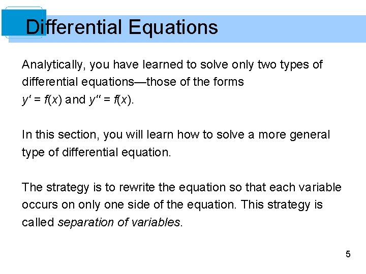
Differential Equations Analytically, you have learned to solve only two types of differential equations—those of the forms y' = f(x) and y'' = f(x). In this section, you will learn how to solve a more general type of differential equation. The strategy is to rewrite the equation so that each variable occurs on only one side of the equation. This strategy is called separation of variables. 5

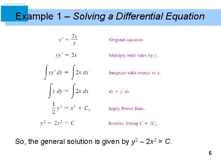
Example 1 – Solving a Differential Equation So, the general solution is given by y 2 – 2 x 2 = C. 6

Growth and Decay Models 7

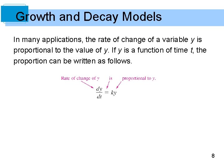
Growth and Decay Models In many applications, the rate of change of a variable y is proportional to the value of y. If y is a function of time t, the proportion can be written as follows. 8

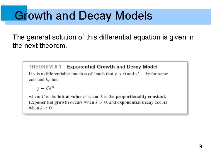
Growth and Decay Models The general solution of this differential equation is given in the next theorem. 9

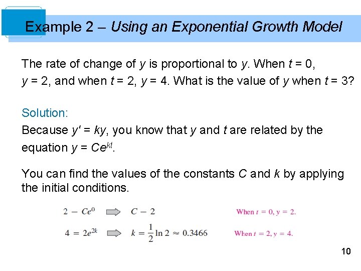
Example 2 – Using an Exponential Growth Model The rate of change of y is proportional to y. When t = 0, y = 2, and when t = 2, y = 4. What is the value of y when t = 3? Solution: Because y' = ky, you know that y and t are related by the equation y = Cekt. You can find the values of the constants C and k by applying the initial conditions. 10

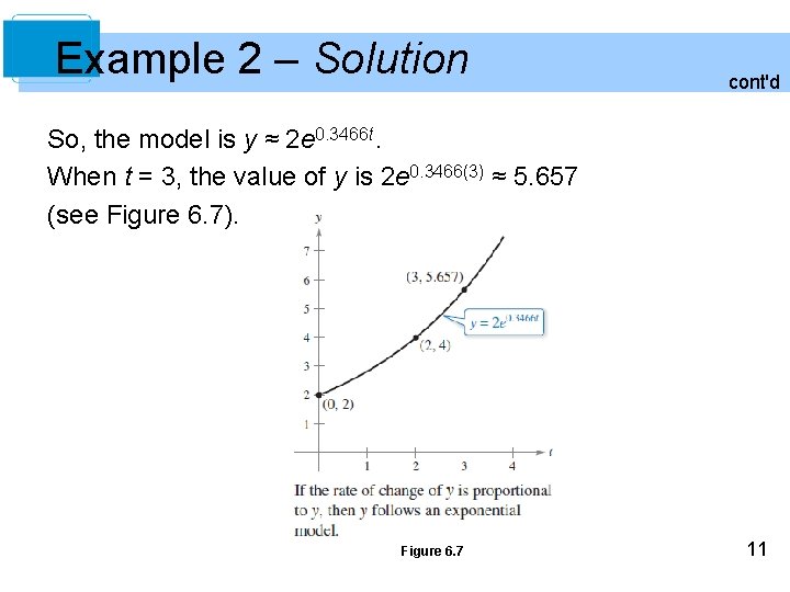
Example 2 – Solution cont'd So, the model is y ≈ 2 e 0. 3466 t. When t = 3, the value of y is 2 e 0. 3466(3) ≈ 5. 657 (see Figure 6. 7). Figure 6. 7 11

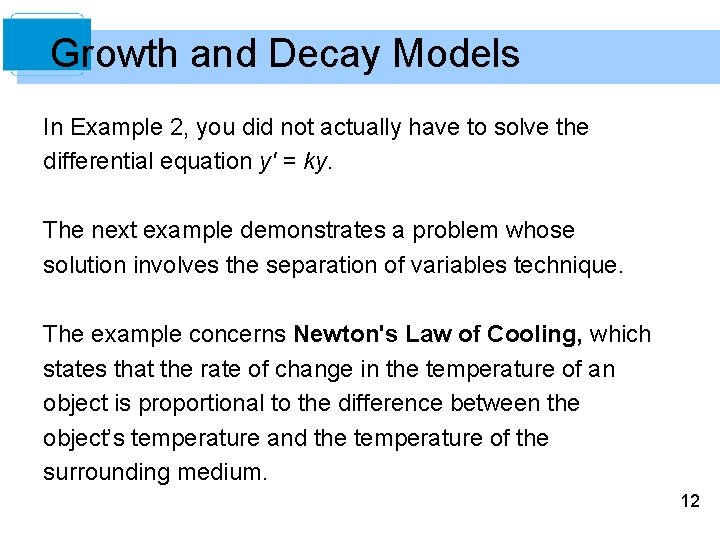
Growth and Decay Models In Example 2, you did not actually have to solve the differential equation y' = ky. The next example demonstrates a problem whose solution involves the separation of variables technique. The example concerns Newton's Law of Cooling, which states that the rate of change in the temperature of an object is proportional to the difference between the object’s temperature and the temperature of the surrounding medium. 12

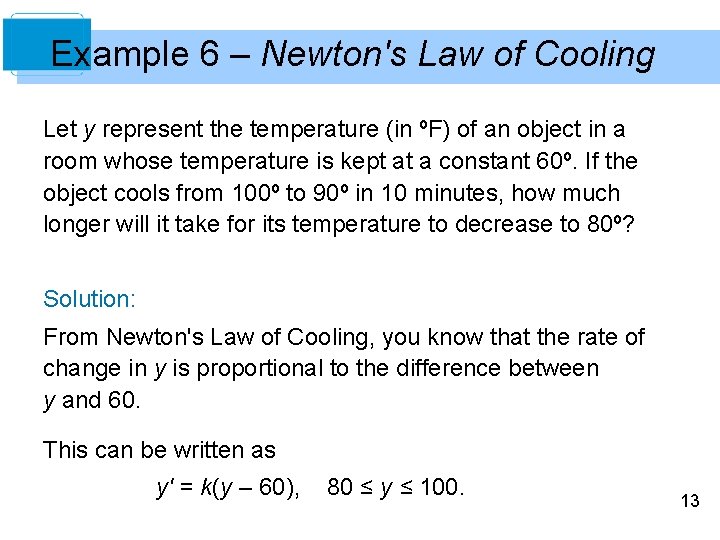
Example 6 – Newton's Law of Cooling Let y represent the temperature (in ºF) of an object in a room whose temperature is kept at a constant 60º. If the object cools from 100º to 90º in 10 minutes, how much longer will it take for its temperature to decrease to 80º? Solution: From Newton's Law of Cooling, you know that the rate of change in y is proportional to the difference between y and 60. This can be written as y' = k(y – 60), 80 ≤ y ≤ 100. 13

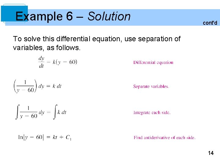
Example 6 – Solution cont'd To solve this differential equation, use separation of variables, as follows. 14

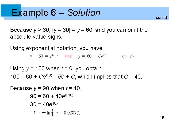
Example 6 – Solution cont'd Because y > 60, |y – 60| = y – 60, and you can omit the absolute value signs. Using exponential notation, you have Using y = 100 when t = 0, you obtain 100 = 60 + Cek(0) = 60 + C, which implies that C = 40. Because y = 90 when t = 10, 90 = 60 + 40 ek(10) 30 = 40 e 10 k 15

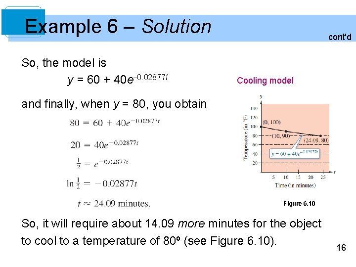
Example 6 – Solution So, the model is y = 60 + 40 e– 0. 02877 t cont'd Cooling model and finally, when y = 80, you obtain Figure 6. 10 So, it will require about 14. 09 more minutes for the object to cool to a temperature of 80º (see Figure 6. 10). 16