Differential Entropy Continuous Random Variable We introduce the

Differential Entropy

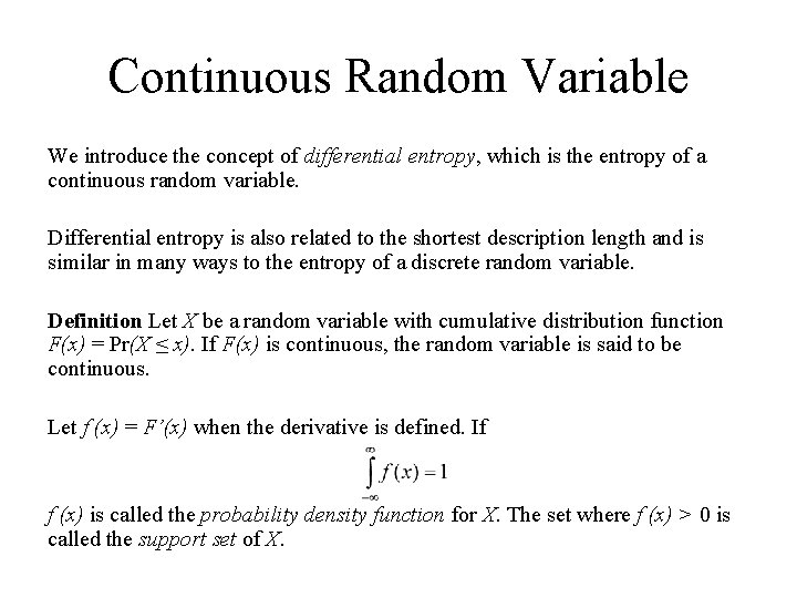
Continuous Random Variable We introduce the concept of differential entropy, which is the entropy of a continuous random variable. Differential entropy is also related to the shortest description length and is similar in many ways to the entropy of a discrete random variable. Definition Let X be a random variable with cumulative distribution function F(x) = Pr(X ≤ x). If F(x) is continuous, the random variable is said to be continuous. Let f (x) = F’(x) when the derivative is defined. If f (x) is called the probability density function for X. The set where f (x) > 0 is called the support set of X.

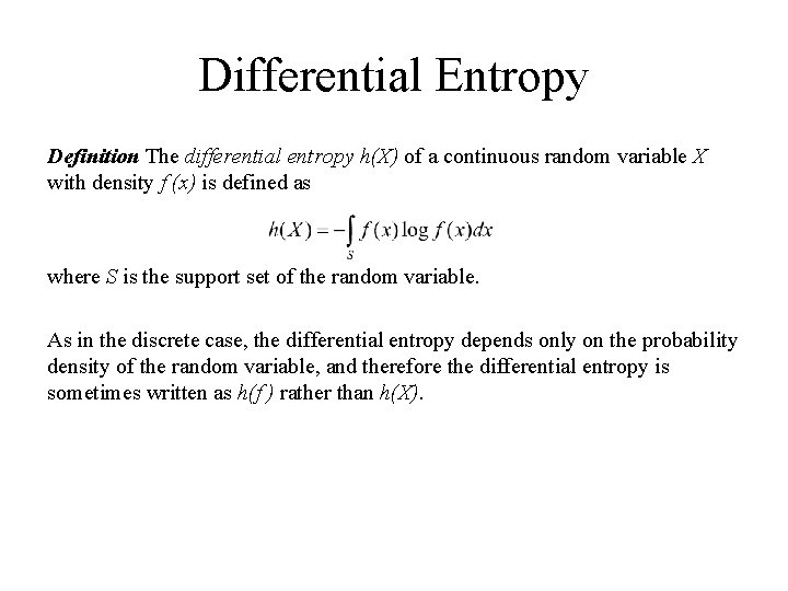
Differential Entropy Definition The differential entropy h(X) of a continuous random variable X with density f (x) is defined as where S is the support set of the random variable. As in the discrete case, the differential entropy depends only on the probability density of the random variable, and therefore the differential entropy is sometimes written as h(f ) rather than h(X).

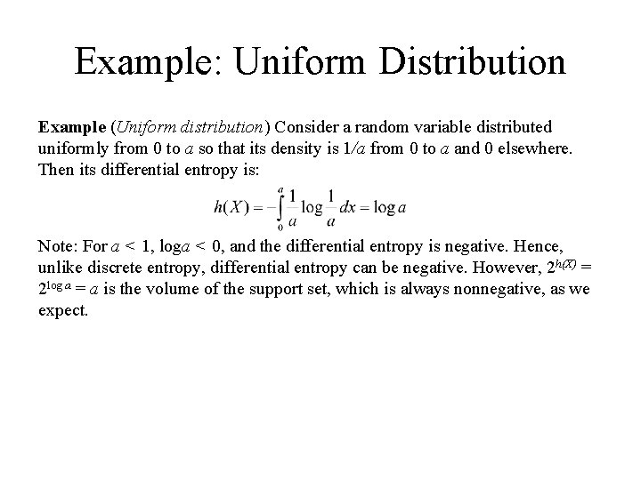
Example: Uniform Distribution Example (Uniform distribution) Consider a random variable distributed uniformly from 0 to a so that its density is 1/a from 0 to a and 0 elsewhere. Then its differential entropy is: Note: For a < 1, loga < 0, and the differential entropy is negative. Hence, unlike discrete entropy, differential entropy can be negative. However, 2 h(X) = 2 log a = a is the volume of the support set, which is always nonnegative, as we expect.

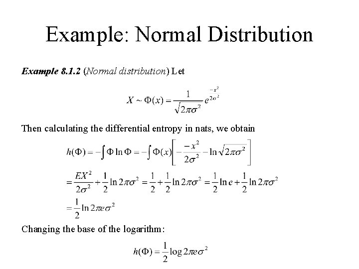
Example: Normal Distribution Example 8. 1. 2 (Normal distribution) Let Then calculating the differential entropy in nats, we obtain Changing the base of the logarithm:

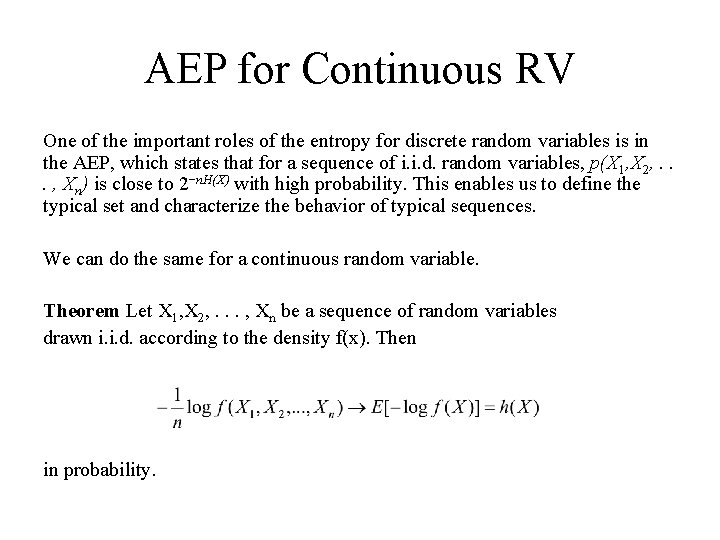
AEP for Continuous RV One of the important roles of the entropy for discrete random variables is in the AEP, which states that for a sequence of i. i. d. random variables, p(X 1, X 2, . . . , Xn) is close to 2−n. H(X) with high probability. This enables us to define the typical set and characterize the behavior of typical sequences. We can do the same for a continuous random variable. Theorem Let X 1, X 2, . . . , Xn be a sequence of random variables drawn i. i. d. according to the density f(x). Then in probability.

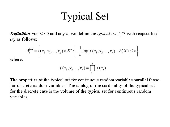
Typical Set Definition For ε> 0 and any n, we define the typical set Aε(n) with respect to f (x) as follows: where: The properties of the typical set for continuous random variables parallel those for discrete random variables. The analog of the cardinality of the typical set for the discrete case is the volume of the typical set for continuous random variables.

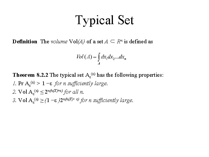
Typical Set Definition The volume Vol(A) of a set A ⊂ Rn is defined as Theorem 8. 2. 2 The typical set Aε(n) has the following properties: 1. Pr Aε(n) > 1 −ε for n sufficiently large. 2. Vol Aε(n) ≤ 2 n(h(X)+ε) for all n. 3. Vol Aε(n) ≥ (1 −ε )2 n(h(X)− ε) for n sufficiently large.

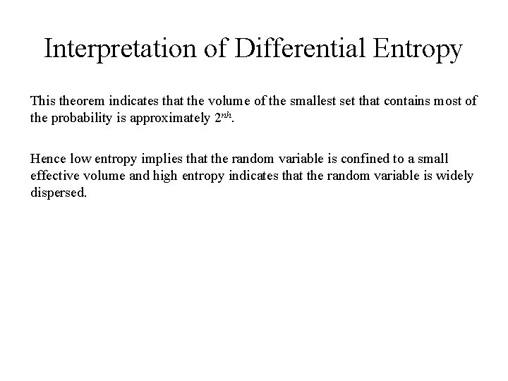
Interpretation of Differential Entropy This theorem indicates that the volume of the smallest set that contains most of the probability is approximately 2 nh. Hence low entropy implies that the random variable is confined to a small effective volume and high entropy indicates that the random variable is widely dispersed.

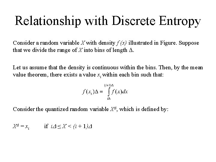
Relationship with Discrete Entropy Consider a random variable X with density f (x) illustrated in Figure. Suppose that we divide the range of X into bins of length . Let us assume that the density is continuous within the bins. Then, by the mean value theorem, there exists a value xi within each bin such that: Consider the quantized random variable X , which is defined by: X = xi if i ≤ X < (i + 1)

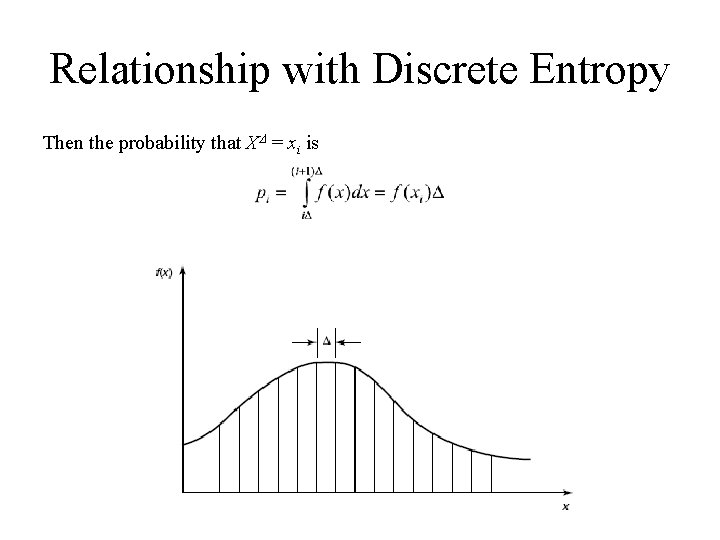
Relationship with Discrete Entropy Then the probability that X = xi is

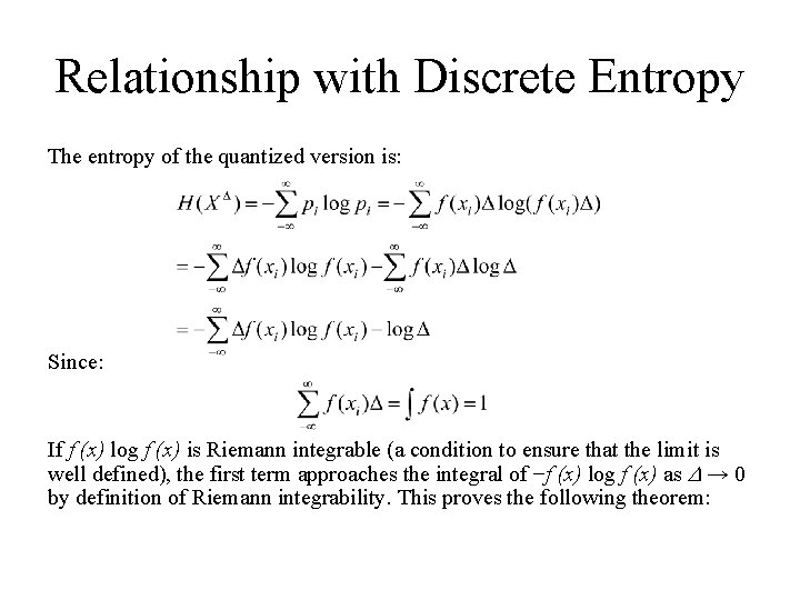
Relationship with Discrete Entropy The entropy of the quantized version is: Since: If f (x) log f (x) is Riemann integrable (a condition to ensure that the limit is well defined), the first term approaches the integral of −f (x) log f (x) as → 0 by definition of Riemann integrability. This proves the following theorem:

Relationship with Discrete Entropy Theorem If the density f(x) of the random variable X is Riemann integrable, then H(X ) + log → h(f ) = h(X), as → 0. Thus, the entropy of an n-bit quantization of a continuous random variable X is approximately h(X) + n.

Examples 1. If X has a uniform distribution on [0, 1] and we let = 2−n, then h = 0, H(X ) = n, and n bits suffice to describe X to n bit accuracy. 2. If X is uniformly distributed on [0, 1/8], the first 3 bits to the right of the decimal point must be 0. To describe X to n-bit accuracy requires only n − 3 bits, which agrees with h(X) = − 3. 3. If X ∼ N(0, σ2) with σ2 = 100, describing X to n bit accuracy would require on the average n + 1/2 log(2πeσ2) = n + 5. 37 bits. In general, h(X) + n is the number of bits on the average required to describe X to n-bit accuracy. The differential entropy of a discrete random variable can be considered to be −∞. Note that 2−∞ = 0, agreeing with the idea that the volume of the support set of a discrete random variable is zero.

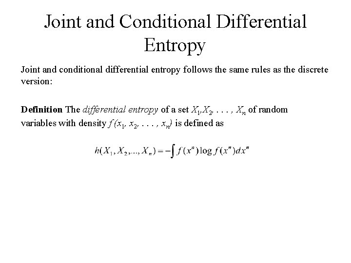
Joint and Conditional Differential Entropy Joint and conditional differential entropy follows the same rules as the discrete version: Definition The differential entropy of a set X 1, X 2, . . . , Xn of random variables with density f (x 1, x 2, . . . , xn) is defined as

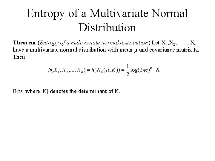
Entropy of a Multivariate Normal Distribution Theorem (Entropy of a multivariate normal distribution) Let X 1, X 2, . . . , Xn have a multivariate normal distribution with mean µ and covariance matrix K. Then Bits, where |K| denotes the determinant of K.

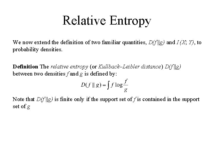
Relative Entropy We now extend the definition of two familiar quantities, D(f ||g) and I (X; Y), to probability densities. Definition The relative entropy (or Kullback–Leibler distance) D(f ||g) between two densities f and g is defined by: Note that D(f ||g) is finite only if the support set of f is contained in the support set of g

Mutual Information Definition The mutual information I (X; Y) between two random variables with joint density f (x, y) is defined as: From the definition it is clear that: I (X; Y) = h(X) − h(X|Y) = h(Y ) − h(Y |X) = h(X) + h(Y ) − h(X, Y ) and I (X; Y) = D(f (x, y)||f (x)f (y)).

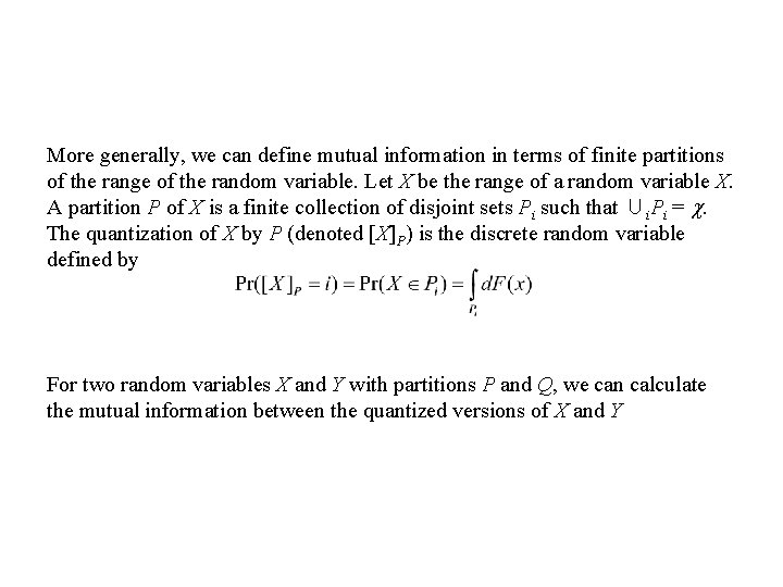
More generally, we can define mutual information in terms of finite partitions of the range of the random variable. Let X be the range of a random variable X. A partition P of X is a finite collection of disjoint sets Pi such that ∪i. Pi = . The quantization of X by P (denoted [X]P) is the discrete random variable defined by For two random variables X and Y with partitions P and Q, we can calculate the mutual information between the quantized versions of X and Y

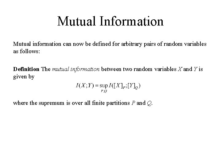
Mutual Information Mutual information can now be defined for arbitrary pairs of random variables as follows: Definition The mutual information between two random variables X and Y is given by where the supremum is over all finite partitions P and Q.

Mutual Information between Correlated Gaussian RV Example (Mutual information between correlated Gaussian random variables with correlation ρ) Let (X, Y) ∼ N(0, K), where: Then h(X) = h(Y ) = 1/2 log(2πe)σ2 and h(X, Y ) = 1/2 log(2πe)2|K| = 1/2 log(2πe)2σ4(1 − ρ2), and therefore I (X; Y) = h(X) + h(Y ) − h(X, Y ) = − 1/2 log(1 − ρ2). If ρ = 0, X and Y are independent and the mutual information is 0. If ρ = ± 1, X and Y are perfectly correlated and the mutual information is infinite.

Summary

More Properties 2 n. H(X) is the effective alphabet size for a discrete random variable. 2 nh(X) is the effective support set size for a continuous random variable. 2 C is the effective alphabet size of a channel of capacity C.