DIFAX Maps DIFAX maps are weather maps generated


")
 • Isobar analysis: – 4 mb increments labeled with tens and")


 •")


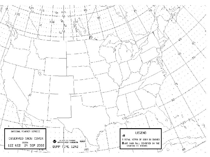
 Depicts snow cover")


 – 30 m intervals with 1500 m")


 – 30 m intervals with 3000 m")

 • Isoheights (solid contours) – 60 m intervals with")
 • Uses: – Wave pattern in the westerlies •")
 • Contains the same contours as the 500 mb North")
 – 120 m intervals with 9000 m")
 – 20 knot intervals with a")

 – 120 m intervals with 10, 000")
 – 20 knot intervals with a")

- Slides: 57
DIFAX Maps • DIFAX maps are weather maps generated by the National Weather Service. • Before the Internet or AWIPS, these were the basic weather analysis and forecast charts used by meteorologists. • They were only available through a fax machine connected to a dedicated landline. • The cost of the landline was very expensive and the special wet electro-conductive paper was expensive; thus only the FAA, NWS, and selective universities and TV stations had access to this information.
• The images were actually burned onto the special FAX paper by electrical currents in the FAX machine. • The rotating helical blade in the fax machine which conducted the electricity to the paper was a deadly weapon: – It was as sharp as a razor and many a person was sliced open by this blade while changing paper rolls or changing the blade itself.
• DIFAX maps, although gradually being phased out, are still available on the internet. • These maps are still unique and contain information which is priceless for operational meteorologists. • All students of meteorology & forecasting will benefit from knowledge of these maps and their interpretation. • Essentially, if you understand how to interpret a black&white DIFAX chart, you should have no problem interpreting pretty colored charts from other sources.
DIFAX Map Descriptions DIFAX maps fall under 2 general categories • Basic data and analysis products – Plotted data – Analyses of basic variables • Forecast products – (generally produced at NCEP) We will concentrate on the first category.
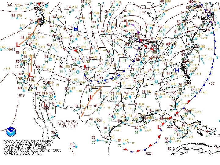
Surface Charts • Analyzed charts issued every 3 hours (0000 Z - 2100 Z) (http: //www. hpc. ncep. noaa. gov/html/about_sfc. shtml) • Data includes – hourly synoptic stations – ship reports – buoy reports • (Maps may be found at the Hydrological Prediction Center) – http: //www. hpc. ncep. noaa. gov/html/sfc 2. shtml • Plotted data example – http: //www. hpc. ncep. noaa. gov/html/stationplot. shtml
Surface Charts (continued) • Isobar analysis: – 4 mb increments labeled with tens and units digit (96, 00, 04, etc. . . ) – Lows and Highs labeled with L and H with the pressure value labeled nearby (in whole mb) • Frontal Analysis – http: //www. hpc. ncep. noaa. gov/html/fntcodes 2. s html • Use: – Current depiction of surface weather features (most valuable weather chart)
Plotted Data Only • Plotted data is available hourly from the HPC – http: //www. hpc. ncep. noaa. gov/sfcobs/sfcobs. shtml
Aviation Surface Analyses • Contains analyzed surface charts and plots. – http: //www. hpc. ncep. noaa. gov/html/avnsfc. shtml • Plots show only the temperature, wind, cloud cover, current weather, and cloud ceiling. – http: //www. hpc. ncep. noaa. gov/html/stationplot_awc. shtml
DIFAX Map Access: • Many DIFAX maps are no longer available, however some of the more important maps are still being produced. • They can be found at: – South Alabama Synoptic Page – www. southalabama. edu/meteorologyclub/synoptic/ National Weather Service: – http: //weather. noaa. gov/fax/nwsfax. html SUNY Albany – http: //www. atmos. albany. edu/weather/difax. html
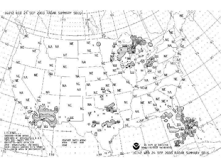
DIFAX Radar Composite Analysis • Gridded from individual radars on a grid (grid spacing roughly 48 km at 60 N) (see overhead) • Entire grid box is assigned the largest value observed anywhere within the grid box (see overhead) • Shading represents echo areas • Contours are incremented Level 1 -3 -5 on a scale of 0 -6. (VIP Levels)
• Echo Tops (tens & hundreds digit truncated: 540=54, 000 ft top) • Echo bases (tens & hundreds digit truncated: 040=4, 000 ft base) • NE = No Echos • NA = Not Available • Movement of Areas and Lines: – Pennants 540 040 From W at 45 kts • Movement of Cells: – Arrows and speed 45 From the WSW at 45 kts
• Precipitation Type and Change of Intensity R RW TRW S SW TSW ZR + - Rainshower Thunderstorm Snowshower Thunder-snowshower Freezing rain New area/cell or increasing intensity Decreasing intensity
• Special Severe Weather Designations (Note: These are less common with Doppler radar network) HOOK HAIL LEWP WER BWER Hook echo (tornadic mesocyclone) Radar-detected hail Line Echo Wave Pattern (bow echoes) Weak Echo Region Bounded Weak Echo Region (supercell mesocyclone) • Watch Boxes WS: WT: Severe Thunderstorm Watch Tornado Watch
• Radar charts are issued nearly hourly – Distributed approximately 1 h after valid time – Data captured at 35 minutes after the hour • Use – Indicates areal coverage, type, intensity and movement of precipitation
Real-Time Radar and Satellite Links • National Weather Service Doppler Radar – http: //www. srh. noaa. gov/radar/national. html • Geostationary Satellite Imagery: – http: //www. ghcc. msfc. nasa. gov/GOES/
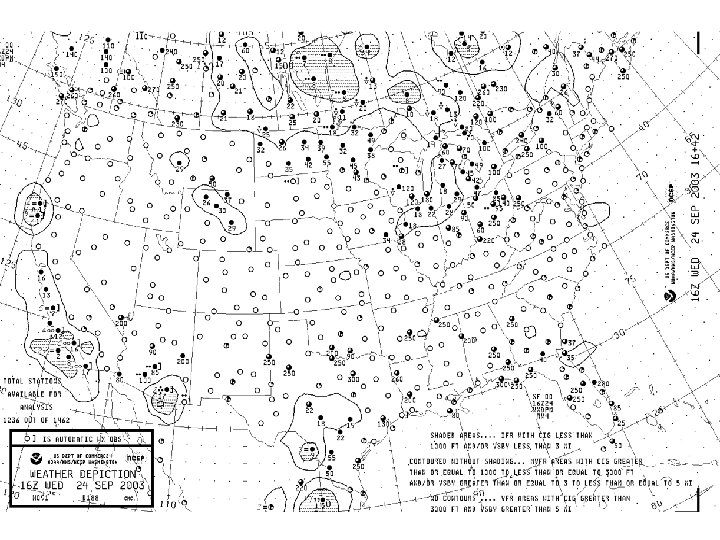
Weather Depiction Chart • Primarily for Aviation-sensitive weather conditions • Issued every 3 hours at 01, 04, 07, 10, 13, 16, 19, & 21 Z) >>> i. e. 1 -hour after synoptic times • Comprised of METAR, cloud, visibility, and current weather information. • Fronts are from the previous hour. • Plotting guide (see handout).
• IFR: Instrument Flight Rules Ceiling < 1000 ft and or Visibility < 3 SM • MVFR: Marginal Visible Flight Rules 1000 ft < ceiling < 3000 ft 3 SM < visibility < 5 SM • VFR: Visual Flight Rules ceiling > 3000 ft visibility > 5 SM
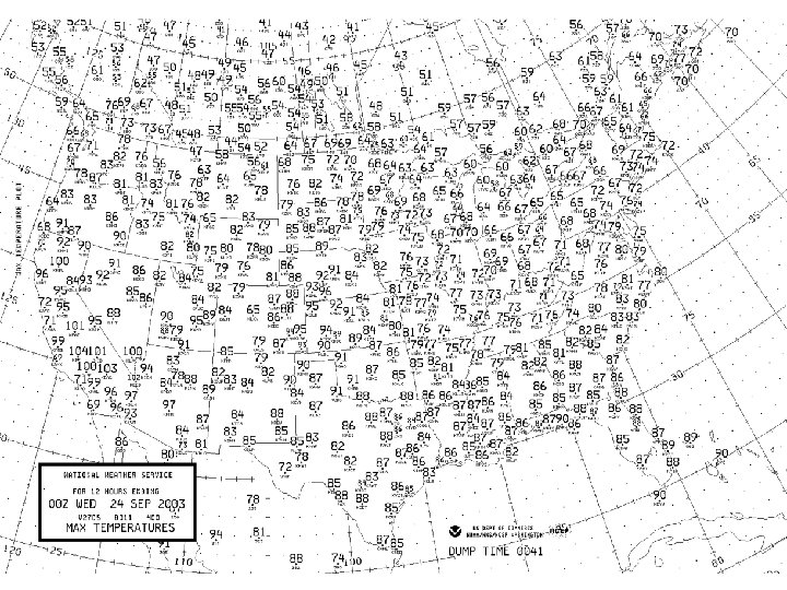
Maximum Temperature Chart • Displays the highest temperatures recorded for the 12 hours prior to 00 Z each day. Time period: (d-1/12 Z - d/00 Z) • Sometimes, the highest temperatures occur at times other than within this 12 -hour window; these occurrences will not be reflected on this chart. – The most common “outside” occurrence of a maximum temperature is heavily influenced by frontal passages.
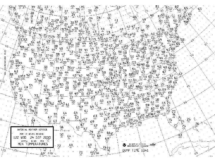
Minimum Temperature Chart • Displays the lowest temperatures recorded for the 12 hours prior to 12 Z each day. Time period: (d/00 Z - d/12 Z) • Sometimes, the lowest daily temperatures occur at times other than within this 12 -hour window; these occurrences will not be reflected on this chart. – The most common “outside” occurrence of a minimum temperature is during the winter shortly after 12 Z. – Frontal influence is also a big factor
Record High and Low Temperatures • Record high and low temperatures are noted on the chart by the l being replaced by a Y. • The type of record is given in the box (situated in the Gulf of Mexico): HI vs LO E: Equalled EX: Exceeded FM: Record for entire month DA: Record for the day
AT: SE: SL: All-time record Record for so early in the year (summer/fall freeze, etc. . . ) Record for so late in the year (spring/summer freeze, etc. . . ) Examples: HIEXDA LOEAT LOEXSE
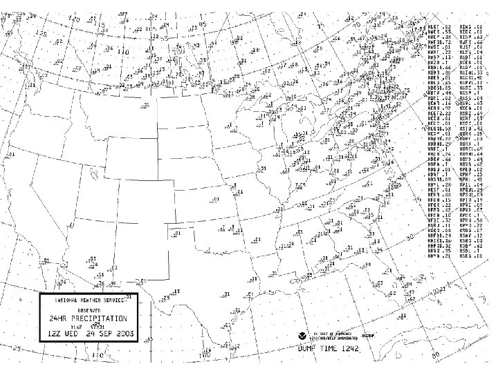
24 Hour Precipitation Chart • Shows liquid-equivalent precipitation totals over a 24 hour period: (d-1/12 Z - d/12 Z) • Precipitation is to the nearest hundredth of an inch. • Inch digit is larger than digits to the right of the decimal. • Additional precipitation totals are printed in the column to the right.
Observed Snow Cover Chart • • Seasonal chart (Sept - April) Depicts snow cover at 12 Z each day Snow cover is in whole inches. Recent accumulations (within the last 6 hours) is depicted by blocked numbers to the right. • Example: 16 9
Upper Air Analysis Charts • Generated every 12 hours with 00 Z and 12 Z data (charts are available on DIFAX 2 to 5 hours after this time). • Produced from the NAM Model analysis – The NAM Model uses a first guess from the previous model run 6 or 12 hours earlier as a basis for constructing the analysis fields. – Data is incorporated into the first-guess field and the analysis is created via Optimal Interpolation (OI) or 4 -D Data Assimilation. – Actual data is plotted on chart, but may not agree with the chart’s analyzed fields.
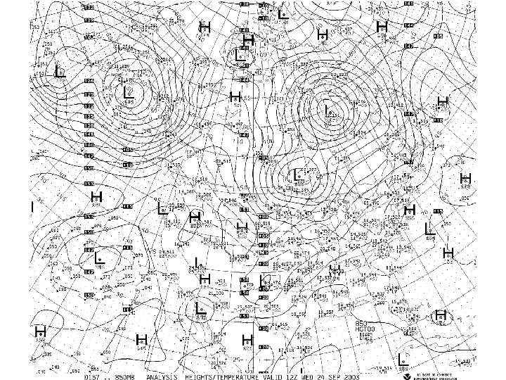
Upper Air Station Model Decoding Heights 850 mb: 150 = 1500 m 700 mb: 300 = 3000 m 500 mb: 540 = 5400 m 300 mb: 900 = 9000 m 250 mb: 000 = 10, 000 m Dewpoint Depression T: -5 C DD: 12 C Td = T – DD Td = -17 C DD < 5 C considered near Sat.
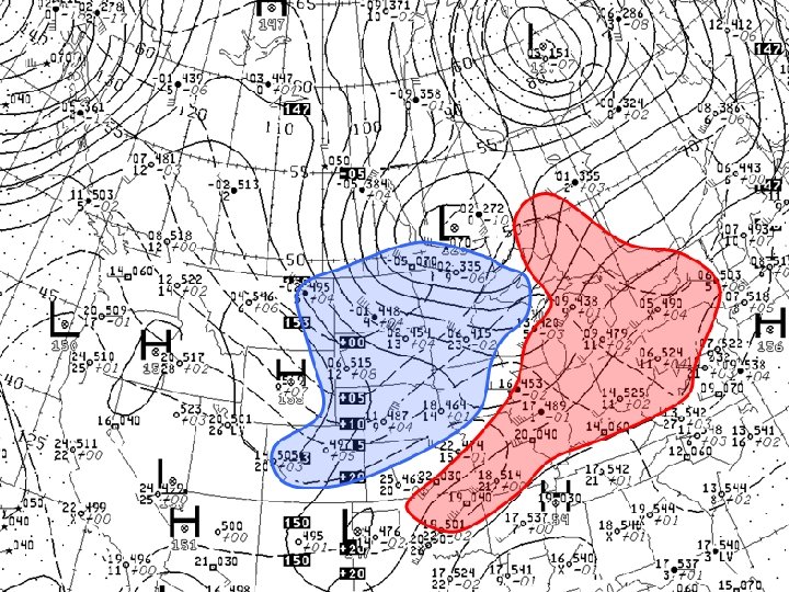
850 mb Chart • Isoheights (solid contours) – 30 m intervals with 1500 m (150 decameters) reference line – contour labels in decameters – plotted heights are in meters (generally add 1 in thousands digit) • Isotherms (dashed contours) – 5 o. C intervals with 0 o. C reference line
850 mb Chart • Uses: – Low Level Jets – Lower tropospheric temperature advection and thermal profile (thermal ridges and troughs) – Lower tropospheric moisture advection and profiles (moist and dry tongues) – Height changes • Caution: – Sometimes underground near high terrain
Thermal Advection • Advection – Horizontal movement of some atmospheric property (Temp, Moisure, Thickness, Vorticity), usually by the wind or atmospheric flow. • Why is Thermal Advection important? – Helps identify the location and movement of fronts – Helps in identifying regions of slantwise upward & downward vertical air motion (tied to isentropic lifting) – Rapid moisture transport can provide additional instability for thunderstorm development.
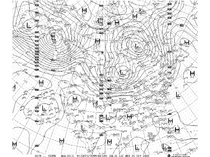
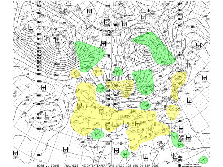
700 mb Chart • Isoheights (solid contours) – 30 m intervals with 3000 m (300 decameters) reference line – contour labels in decameters – plotted heights are in meters (generally add 2 or 3 in thousands digit) • Isotherms (dashed contours) – 5 o. C intervals with 0 o. C reference line
700 mb Chart • Uses: – Elevated tropospheric moisture advection and profiles (elevated dry intrusions; moist tongues) – Mid-tropospheric temperature advection and thermal profile (thermal ridges and troughs) – Mid-level jets – Height changes • Caution: – Sometimes near surface in higher terrain
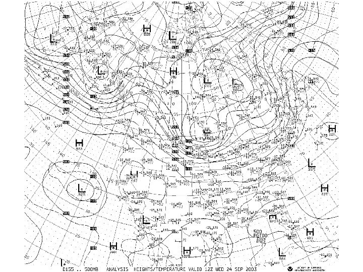
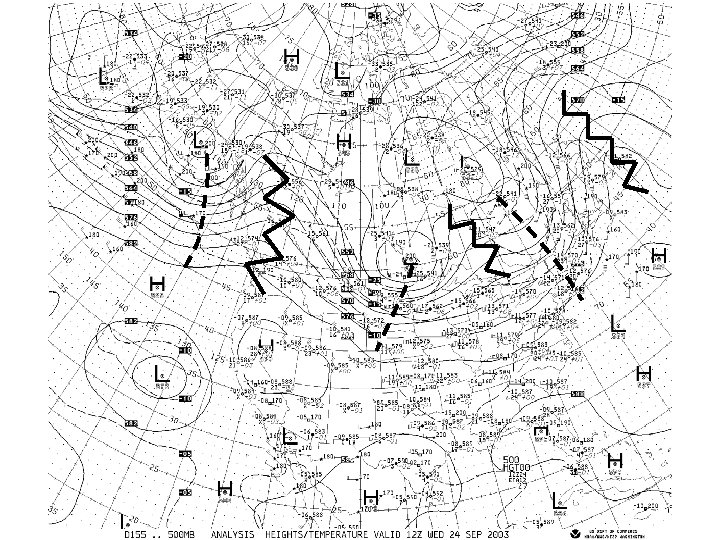
500 mb Chart (North America) • Isoheights (solid contours) – 60 m intervals with 5400 m (540 decameters) reference line – contour labels in decameters – plotted heights are in decameters (add 0 in ones digit for meters) • Isotherms (dashed contours) – 5 o. C intervals with 0 o. C reference line
500 mb Chart (North America) • Uses: – Wave pattern in the westerlies • Identification of longwaves and shortwaves – Height changes and wave motion – Approximate steering level for surface synoptic systems – Vertical and horizontal tilt of waves – Mid-tropospheric temperature advection and thermal profile (warm and cold pools) – Mid-tropospheric moisture profiles
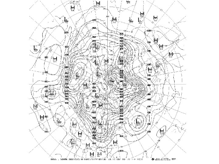
500 mb Chart (Hemispheric) • Contains the same contours as the 500 mb North American analysis, except void of data plots • Additional Uses: – Circumpolar vortex configuration – Planetary wave number and pattern – Wave identification • Internet Address (Environment Canada): – http: //weatheroffice. ec. gc. ca/data/analysis/sai_50. gif
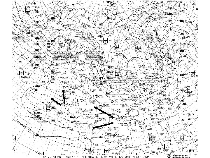
300 mb Analysis • Isoheights (solid contours) – 120 m intervals with 9000 m (900 decameter) reference line – contour labels in decameters – plotted heights are in decameters (add 0 in ones digit for meters) • Isotherms (dashed heavy contours) – 5 o. C intervals with -50 o. C reference line
300 mb Analysis • Isotachs (light dashed contours) – 20 knot intervals with a 10 knot reference line – Stippled regions represent: • 70 -110 knot winds • 150 -190 knot winds
300 mb Analysis • Uses: – Polar jet stream location/configuration/intensity • The 4 -quadrant jet/divergence relationship – Upper-tropospheric wave pattern – Regions of Difluence and Confluence (convection/severe weather) – Regions of upper-tropospheric vertical shear (tropical cyclones)
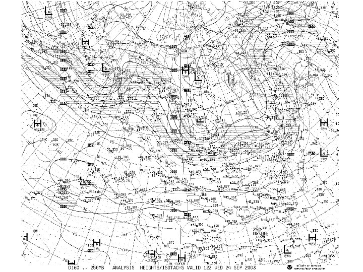
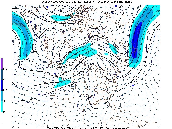
250 mb Analysis • Isoheights (solid contours) – 120 m intervals with 10, 000 m (1000 decameter) reference line – contour labels in decameters – plotted heights are in decameters (add 0 in ones digit for meters, and possibly a 1 for the tenthousands digit [if first plotted number is a 0]) • Isotherms (dashed heavy contours) – 5 o. C intervals with -50 o. C reference line
250 mb Analysis • Isotachs (light dashed contours) – 20 knot intervals with a 10 knot reference line – Stippled regions represent: • 70 -110 knot winds • 150 -190 knot winds
250 mb Analysis • Uses: – Sub-tropical jet stream location/configuration/intensity – the 4 -quadrant jet/divergence relationship – Upper-tropospheric wave pattern – Regions of Difluence and Confluence (convection/severe weather) – Regions of upper-tropospheric vertical shear (tropical cyclones) – Tropopause folds and breaks