DIAGNOSTIC RADIOLOGY Introduction www oghabian net Electromagnetic spectrum

DIAGNOSTIC RADIOLOGY Introduction www. oghabian. net

Electromagnetic spectrum E 1. 5 3 e. V IR light 8000 4000 0. 12 ke. V 1 10 102 ke. V 103 104 X and rays UV 100 10 IR : infrared, UV = ultraviolet 1 0. 01 0. 001 Angström
 E 0 E From a “thin” target")
Bremsstrahlung spectra d. N/d. E (spectral density) E 0 E From a “thin” target E 0= energy of electrons d. N/d. E E 0 E From a “thick” target E = energy of emitted photons

X-ray spectrum energy • Maximum energy of Bremsstrahlung photons – kinetic energy of incident electrons • In X-ray spectrum of radiology installations: – Max (energy) = X-ray tube peak voltage E Bremsstrahlung 50 100 150 200 ke. V Bremsstrahlung after filtration ke. V

Ionization and associated energy transfers Example: electrons in water • ionization energy : 16 e. V (for a water molecule) • other energy transfers associated to ionization – Excitation energy (each requires only a few e. V) – thermal transfers (at even lower energy) • W = 32 e. V is the average loss per ionization – it is characteristic of the medium – independent of incident particle and of its energy
 Energy (e. V) K 1 100 - 20")
Spectral distribution of characteristic X-rays (II) Energy (e. V) K 1 100 - 20 - 70 - 590 - 2800 - 11000 P O N M L - 69510 K 6 5 4 3 2 80 K 2 60 40 L L 20 0 0 K 2 L 10 20 K 1 30 40 50 60 70 80 (ke. V)

Basic elements of the x-ray assembly source • Generator : power circuit supplying the required potential to the X-ray tube • X-ray tube and collimator: device producing the X-ray beam

X-ray tube components 1: mark of focal spot 1: long tungsten filament 2 : short tungsten filament 3 : real size cathode Add module code number and lesson title 8
 • The Line-Focus principle – Anode target plate has a shape")
Anode angle (I) • The Line-Focus principle – Anode target plate has a shape that is more rectangular or ellipsoidal than circular • the shape depends on : – filament size and shape – focusing cup’s and potential – distance between cathode and anode – Image resolution requires a small focal spot – Heat dissipation requires a large spot • This conflict is solved by slanting the target face Add module code number and lesson title 9
 Angle Incident electron beam width Actual focal spot size Incident electron")
Anode angle (II) Angle Incident electron beam width Actual focal spot size Incident electron beam width Apparent focal spot size Angle Actual focal spot size Increased apparent focal spot size Film THE SMALLER THE ANGLE THE BETTER THE RESOLUTION Add module code number and lesson title 10
 • Anode angle (from 7° to 20°) induces a variation")
Anode heel effect (I) • Anode angle (from 7° to 20°) induces a variation of the X-ray output in the plane comprising the anode-cathode axis • Absorption of photons by anode body is more in low emission angle • The magnitude of influence of the heel effect on the image depends on factors such as : – anode angle – size of film (FOV) – focus to film distance • Anode aging increases heel effect Add module code number and lesson title 11

Heat loading capacities • A procedure generates an amount of heat depending on: – k. V used, tube current (m. A), length of exposure – type of voltage waveform – number of exposures taken in rapid sequence • Heat Unit (HU) [joule] : unit of potential x unit of tube current x unit of time • The heat generated by various types of X-ray circuits are: – – 1 phase units : 3 phase units, 6 pulse : 3 phase units, 12 pulse: J = HU x 0. 71 HU = k. V x m. A x s HU = 1. 35 k. V x m. A x s HU = 1. 41 k. V x m. A x s Add module code number and lesson title 12
 Tube current (m. A) 700 X-ray tube B 3")
X-ray tube rating chart (IV) Tube current (m. A) 700 X-ray tube B 3 full-wave rectified 10. 000 rpm 1. 0 mm effective focal spot 600 500 400 300 70 90 k. Vp 50 p k. V p 125 k. V p 200 Acceptable 100 0. 01 0. 05 0. 1 0. 5 1. 0 5. 0 10. 0 Exposure time (s) Add module code number and lesson title 13
 • Heat generated is stored in the anode, and dissipated")
Anode cooling chart (I) • Heat generated is stored in the anode, and dissipated through the cooling circuit • A typical cooling chart has : – input curves (heat units stored as a function of time) – anode cooling curve • The following graph shows that : – a procedure delivering 500 HU/s can go on indefinitely – if it is delivering 1000 HU/s it has to stop after 10 min – if the anode has stored 120. 000 HU, it will take 5 min to cool down. Add module code number and lesson title 14
 Heat units stored (x 1000) 240 Maximum Heat Storage Capacity")
Anode cooling chart (II) Heat units stored (x 1000) 240 Maximum Heat Storage Capacity of Anode ec U/s 0 H 220 100 200 Imput curve ec U/s H 0 50 180 160 140 350 H 120 U/sec ec /s 250 HU 100 Co o 80 lin g 60 cu rve 40 20 1 2 3 4 5 6 7 8 9 10 11 Elapsed time (min) Add module code number and lesson title 12 13 14 15
 • Generator characteristics have a strong influence on the contrast and")
X-ray generator (II) • Generator characteristics have a strong influence on the contrast and sharpness of the radiographic image • The motion unsharpness can be greatly reduced by a generator allowing an exposure time as short as achievable • Since the dose at the image plane can be expressed as : – – D = k 0. k. Vpn. I. T k. Vp : peak voltage (k. V) I : mean current (m. A) T : exposure time (ms) n : ranging from about 3 at 150 k. V to 5 at 50 k. V Add module code number and lesson title 16
 • Peak voltage value has an influence on the beam hardness")
X-ray generator (III) • Peak voltage value has an influence on the beam hardness • It has to be related to medical question – What is the anatomical structure to investigate ? – What is the contrast level needed ? • The ripple “r” of a generator has to be as low as possible r = [(k. V - k. Vmin)/k. V] x 100% Add module code number and lesson title 17
 Single phase single pulse k. V ripple (%) 100%")
Tube potential wave form (II) Single phase single pulse k. V ripple (%) 100% Single phase 2 -pulse 13% Three phase 6 -pulse 4% Three phase 12 -pulse Line voltage 0. 01 s 0. 02 s Add module code number and lesson title 18

Radiation emitted by the x-ray tube • Primary radiation : before interacting photons • Scattered radiation : after at least one interaction • Leakage radiation : not absorbed by the x-ray tube housing shielding • Transmitted radiation : emerging after passage through matter Antiscatter grid

Thin Target X-ray Formation Interestingly, this process creates a relatively uniform spectrum. Maximum energy is created when an electron gives all of its energy, 0 , to one photon. Or, the electron can produce n photons, each with energy 0/n. Or it can produce a number of events in between. Power output is proportional to 0 2 Intensity = nh 0 Photon energy spectrum 20

Thick Target X-ray Formation We can model target as a series of thin targets. Electrons successively loses energy as they moves deeper into the target. Gun X-rays Relative Intensity 11/24/2020 0 Each layer produces a flat energy spectrum with decreasing peak energy level. 21

Stopping power *Loss of energy along track through collisions *The linear stopping power of the medium S = E / x [Me. V. cm-1] • • E: energy loss x: element of track *for distant collisions : the lower the electron energy, the higher the amount transferred *most Bremsstrahlung photons are of low energy *collisions (hence ionization) are the main source of energy loss *except at high energies or in media of high Z
 Energy (e. V) - 20 - 70 -")
Spectral distribution of characteristic X-rays (II) Energy (e. V) - 20 - 70 - 590 - 2800 - 11000 P O N M L - 69510 K 11/24/2020 K 1 100 6 5 4 3 2 80 K 2 60 40 L L 20 0 0 K 2 L 10 20 K 1 30 40 50 60 70 80 (ke. V) 23

Thick Target X-ray Formation Andrew Webb, Introduction to Biomedical Imaging, 2003, Wiley. Interscience. ( Lower energy photons are absorbed with aluminum to block radiation that will be absorbed by surface of body and won’t contribute to image. The photoelectric effect will create significant spikes of energy when accelerated 11/24/2020 electrons collide with tightly bound electrons, usually in the K shell. 24

Factors influencing the x-ray spectrum • tube potential – k. Vp value • wave shape of tube potential • anode track material – W, Mo, Rh etc. • X-ray beam filtration – inherent + additional Number of photons (arbitrary normalisation) X-ray spectrum at 30 k. V for an X-ray tube with a Mo target and a 0. 03 mm Mo filter 15 10 Add module code number and lesson title 15 20 25 Energy (ke. V) 30 25

Automatic exposure control • Optimal choice of technical parameters in order to avoid repeated exposures (k. V, m. A) • Radiation detector behind (or in front of) the film cassette (with due correction) • Exposure is terminated when the required dose has been integrated • Compensation for k. Vp at a given thickness • Compensation for thickness at a given k. Vp

Interaction of radiation with matter Radiation Contrast
:")
Linear Energy Transfer • Biological effectiveness of ionizing radiation • Linear Energy Transfer (LET): amount of energy transferred to the medium per unit of track length of the particle • Unit : e. g. [ke. V. m-1]
 Matter is composed")
How do we describe attenuation of X-rays by body? Assumptions: 1) Matter is composed of discrete particles (i. e. electrons, nucleus) 2) Distance between particles >> particle size 3) X-ray photons are small particles Interact with body in binomial process Pass through body with probability p Interact with body with probability 1 -p (Absorption or scatter) 11/24/2020 29
 number of xray photons N and ∆x. N |")
The number of interactions (removals=∆N) number of xray photons N and ∆x. N | ∆x | N - ∆N Nin x Nout µ ∆N = -µN∆x µ = f(Z, ) Attenuation a function of atomic number Z and energy Solving the differential equation: Nout ∫ N x d. N/N = -µ ∫ dx in 0 d. N = -µNdx ln (Nout/Nin) = -µx Nout = Nin e-µx 30 11/24/2020
 Nout =")
If material attenuation varies in x, we can write attenuation as µ(x) Nout = Nin e -∫µ(x) dx If Io photons/cm 2 Id (x, y) (µ (x, y, z)) Detector Plane Id (x, y) = I 0 exp [ -∫ µ(x, y, z) dz] Assume: perfectly collimated beam ( for now), perfect detector no loss of resolution 11/24/2020 31

Actually recall that attenuation is also a function of energy , µ = µ(x, y, z, ) Id (x, y) = ∫ I 0 ( ) exp [ -∫ µ (x, y, z, ) dz] d Which Integrate over and depth. For a single energy I 0( ) = I 0 ( - o) = I 0 After analyzing a single energy, we can add the effects of other energies by superposition. If homogeneous material, then µ (x, y, z, 0) = µ 0 Id (x, y) = I 0 e -µ 0∆z 11/24/2020 32

Attenuation of an heterogeneous beam • Various energies No more exponential attenuation • Progressive elimination of photons through the matter • Lower energies preferentially • This effect is used in the design of filters • Beam hardening effect 11/24/2020 33
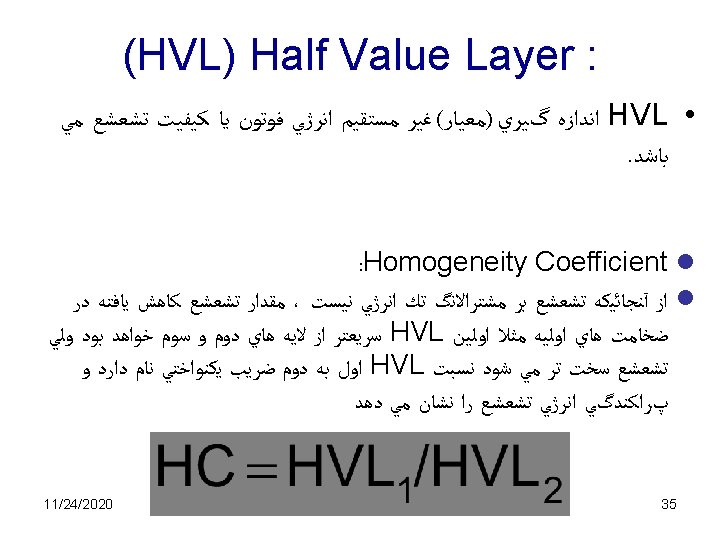
 • HVL: thickness reducing beam intensity by 50% • Definition")
Half Value Layer (HVL) • HVL: thickness reducing beam intensity by 50% • Definition holds strictly for monoenergetic beams • • Heterogeneous beam hardening effect I/I 0 = 1/2 = exp (-µ HVL) HVL = 0. 693 / µ HVL depends on material and photon energy HVL characterizes beam quality • modification of beam quality through filtration • HVL (filtered beam) HVL (beam before filter) 11/24/2020 34

X-ray interaction with matter Coherent Scattering Photoelectric Effect Compton Scattering Pair Production Photodisintegration. Add module code number and lesson title 36

Coherent Scattering - Rayleigh • • Coherent scattering varies over diagnostic energy range as: • • • 2 µ/p 1/ • 11/24/2020 37

Photoelectric effect • Incident photon with energy h • Absorption: all photon energy absorbed by a tightly bound orbital electron ejection of electron from the atom • • Kinetic energy of ejected electron : E = h - EB Condition : h > EB (electron binding energy) Recoil of the residual atom Attenuation (or interaction): photoelectric absorption coefficient

We can use K-edge to dramatically increase absorption in areas where material is injected, ingested, etc. ln /r K edge 11/24/2020 Log ( ) Photon energy 39

Compton scattering • Interaction between photon and electron • h = Ea + Es (energy is conserved) – Ea: energy transferred to the atom – Es : energy of the scattered photon – momentum is conserved in angular distributions • Compton is practically independent of Z in diagnostic range • The probability of interaction decreases as h increases • Compton effect is proportional to the electron density in the medium

- Interaction of photons and electrons produce scattered photons of reduced energy. - The probability of interaction decreases as h increases -Compton effect is proportional to the electron density in the medium E’ photon E 11/24/2020 Outer Shell electron E=h = E’+Ee v Electron (“recoil”) 41
c 2= increase in electron energy} (Mass of moving")
Satisfy Conservation of Energy: {(m-mo )c 2= increase in electron energy} (Mass of moving electron) Conservation of Momentum in x and y direction: E’ photon E v Electron (“recoil”) 42

Energy of Compton or recoil electron ∆E: change in energy of photon change in wavelength of photon h = 6. 63 x 10 -34 Jsec e. V = 1. 62 x 10 -19 J mo = 9. 31 x 10 -31 kg ∆ = h/ moc (1 - cos ) = 0. 0241 A 0 (1 - cos ) ∆ at = π = 0. 048 Angstroms Energy of Compton photon: 43

Rayleigh, Compton, Photoelectric are independent sources of attenuation t = I/I 0 = e-µl = exp [ -(µc + µR + µp)l] µ( ) ≈ r. Ng {Cc(1/ ) + CR (Z 2/ 1. 9) + Cp (Z 3. 8/ 3. 2)} Compton Rayleigh Photoelectric Mass attenuation coefficient (µ/r) electron mass density Ng Ng = electrons/gram r. Ng = electrons/cm 3 Ng = NA (Z/A) ≈ NA /2 (all but H) A = atomic mass NA =6. 0 x 1023 Unfortunately, almost all elements have electron mass density ≈ 3 x 10 23 electrons/gram Hydrogen (exception) ≈ 6. 0 x 1023 electrons/gram 44

Attenuation Mechanisms Curve on left shows how photoelectric effects dominates at lower energies and how Compton effect dominates at higher energies. Curve on right shows that mass attenuation coefficient varies little over 100 kev. Ideally, we would image at lower energies to create contrast.

Photoelectric vs. Compton Effect The curve above shows that the Compton effect dominates at higher energy values as a function of atomic number. Ideally, we would like to use lower energies to use the higher contrast available with 11/24/2020 46 The photoelectric effect. Higher energies are needed however as the body gets thicker.

Scattered radiation • Effect on mage quality – increasing of blurring – loss of contrast • Effect on patient dose – increasing of superficial and depth dose Possible reduction through : use of grid limitation of the field to the useful portion limitation of the irradiated volume (e. g. : breast compression in mammography) Higher k. Vp
 Incident photons")
Photon interactions with matter Scattered photon Compton effect Fluorescence photon (Characteristic radiation) Incident photons Annihilation photon Recoil electron Photoelectron (Photoelectric effect) Electron pair E > 1. 02 Me. V Secondary photons Non interacting photons Secondary electrons (simplified representation)
- Slides: 50