Developmental models Multivariate analysis choleski models factor models

Developmental models

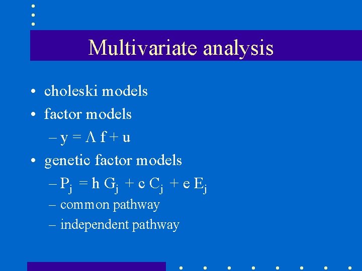
Multivariate analysis • choleski models • factor models –y= f+u • genetic factor models – Pj = h Gj + c C j + e E j – common pathway – independent pathway

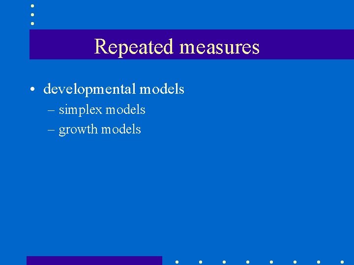
Repeated measures • developmental models – simplex models – growth models

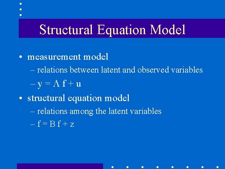
Structural Equation Model • measurement model – relations between latent and observed variables –y= f+u • structural equation model – relations among the latent variables –f=Bf+z

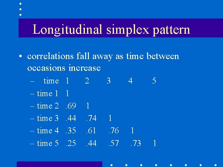
Longitudinal simplex pattern • correlations fall away as time between occasions increase – time 1 – time 2 – time 3 – time 4 – time 5 1 1. 69. 44. 35. 25 2 3 4 5 1. 74. 61. 44 1. 76. 57 1. 73 1

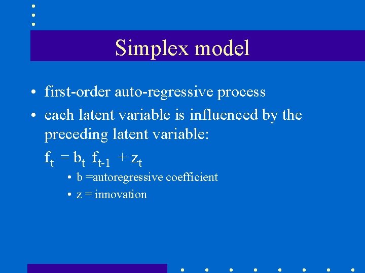
Simplex model • first-order auto-regressive process • each latent variable is influenced by the preceding latent variable: ft = bt ft-1 + zt • b =autoregressive coefficient • z = innovation

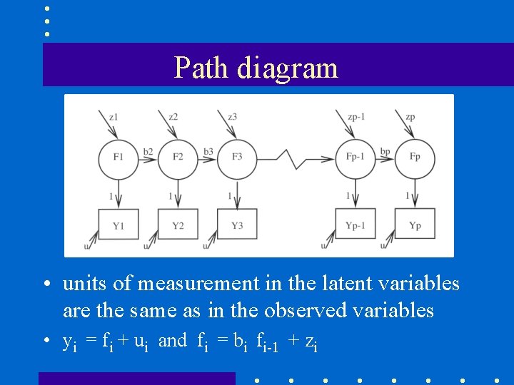
Path diagram • units of measurement in the latent variables are the same as in the observed variables • yi = fi + ui and fi = bi fi-1 + zi

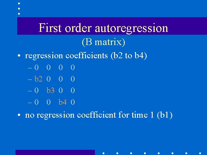
First order autoregression (B matrix) • regression coefficients (b 2 to b 4) – 0 – b 2 – 0 0 0 b 3 0 0 b 4 0 0 • no regression coefficient for time 1 (b 1)

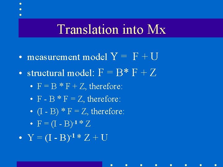
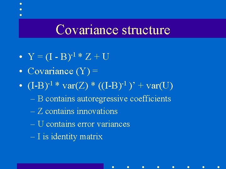
Translation into Mx • measurement model Y = F + U • structural model: F = B* F + Z • • F = B * F + Z, therefore: F - B * F = Z, therefore: (I - B) * F = Z, therefore: F = (I - B)-1 * Z • Y = (I - B)-1 * Z + U

Covariance structure • Y = (I - B)-1 * Z + U • Covariance (Y) = • (I-B)-1 * var(Z) * ((I-B)-1 )’ + var(U) – B contains autoregressive coefficients – Z contains innovations – U contains error variances – I is identity matrix

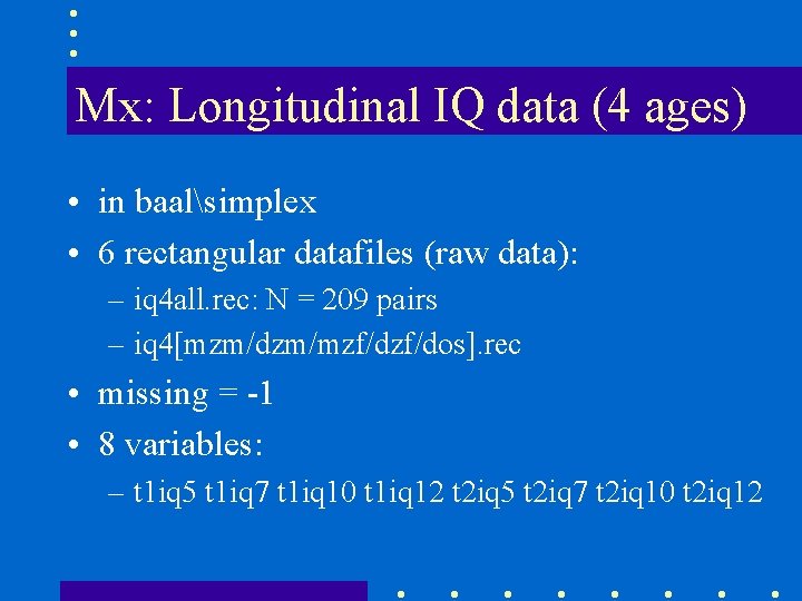
Mx: Longitudinal IQ data (4 ages) • in baalsimplex • 6 rectangular datafiles (raw data): – iq 4 all. rec: N = 209 pairs – iq 4[mzm/dzm/mzf/dos]. rec • missing = -1 • 8 variables: – t 1 iq 5 t 1 iq 7 t 1 iq 10 t 1 iq 12 t 2 iq 5 t 2 iq 7 t 2 iq 10 t 2 iq 12

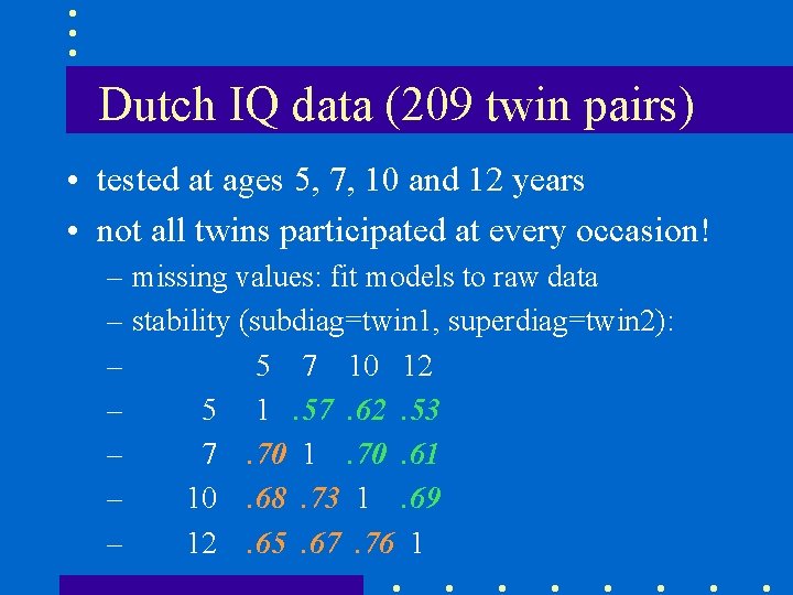
Dutch IQ data (209 twin pairs) • tested at ages 5, 7, 10 and 12 years • not all twins participated at every occasion! – missing values: fit models to raw data – stability (subdiag=twin 1, superdiag=twin 2): – 5 7 10 12 – 5 1. 57. 62. 53 – 7. 70 1. 70. 61 – 10. 68. 73 1. 69 – 12. 65. 67. 76 1

2 Mx jobs • 1 factor: Pfact 4 iq. mx • simplex: Psimp 4 iq. mx • input file: iq 4 all. rec

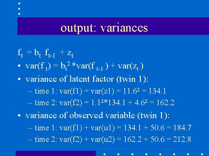
output: variances ft = bt ft-1 + zt • var(f t) = bt 2 *var(f t-1 ) + var(zt ) • variance of latent factor (twin 1): – time 1: var(f 1) = var(z 1) = 11. 62 = 134. 1 – time 2: var(f 2) = 1. 12*134. 1 + 4. 62 = 162. 2 • variance of observed variable (twin 1): – time 1: var(f 1) + var(u 1) = 134. 1 + 50. 6 = 184. 7 – time 2: var(f 2) + var(u 2) = 162. 2 + 50. 6 = 212. 8

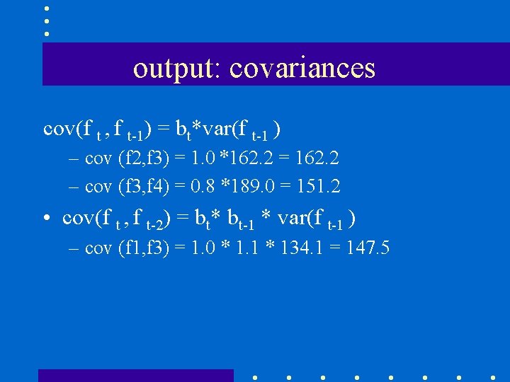
output: covariances cov(f t , f t-1) = bt*var(f t-1 ) – cov (f 2, f 3) = 1. 0 *162. 2 = 162. 2 – cov (f 3, f 4) = 0. 8 *189. 0 = 151. 2 • cov(f t , f t-2) = bt* bt-1 * var(f t-1 ) – cov (f 1, f 3) = 1. 0 * 1. 1 * 134. 1 = 147. 5

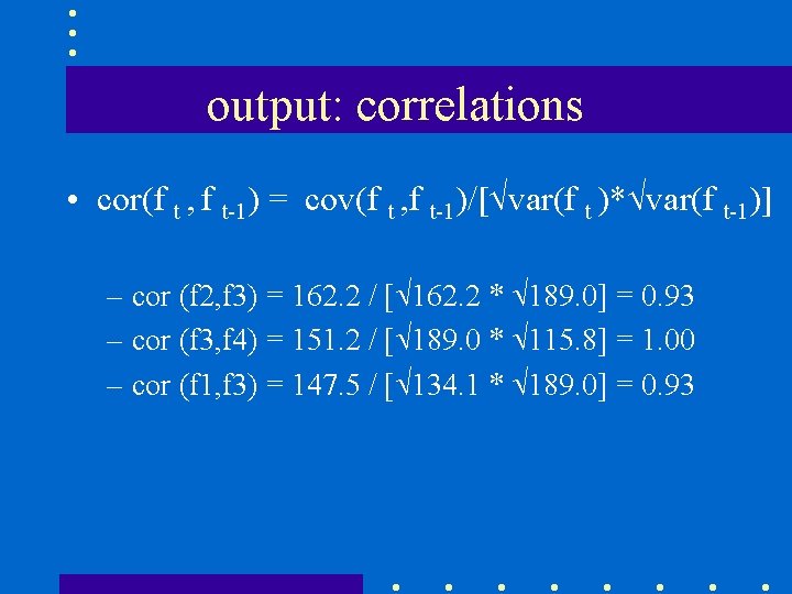
output: correlations • cor(f t , f t-1) = cov(f t , f t-1)/[ var(f t )* var(f t-1)] – cor (f 2, f 3) = 162. 2 / [ 162. 2 * 189. 0] = 0. 93 – cor (f 3, f 4) = 151. 2 / [ 189. 0 * 115. 8] = 1. 00 – cor (f 1, f 3) = 147. 5 / [ 134. 1 * 189. 0] = 0. 93

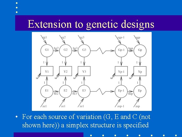
Extension to genetic designs • For each source of variation (G, E and C (not shown here)) a simplex structure is specified

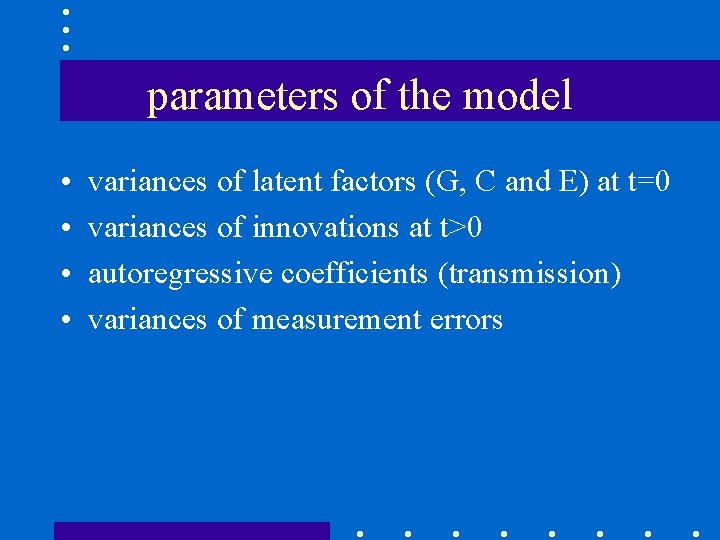
parameters of the model • • variances of latent factors (G, C and E) at t=0 variances of innovations at t>0 autoregressive coefficients (transmission) variances of measurement errors

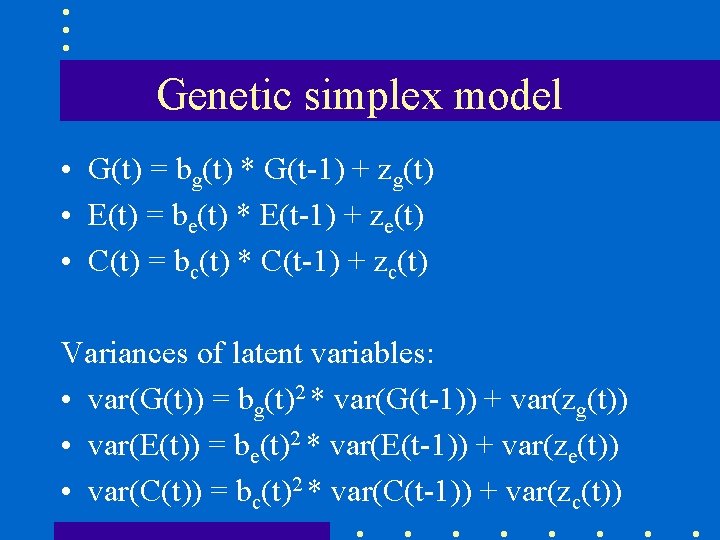
Genetic simplex model • G(t) = bg(t) * G(t-1) + zg(t) • E(t) = be(t) * E(t-1) + ze(t) • C(t) = bc(t) * C(t-1) + zc(t) Variances of latent variables: • var(G(t)) = bg(t)2 * var(G(t-1)) + var(zg(t)) • var(E(t)) = be(t)2 * var(E(t-1)) + var(ze(t)) • var(C(t)) = bc(t)2 * var(C(t-1)) + var(zc(t))

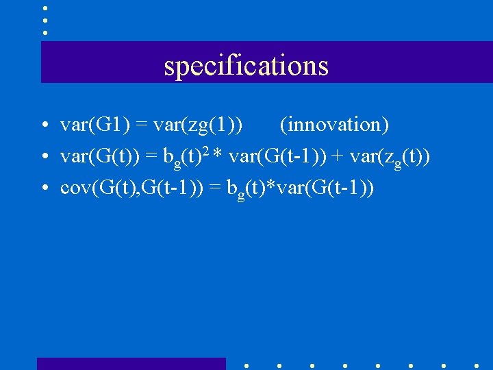
specifications • var(G 1) = var(zg(1)) (innovation) • var(G(t)) = bg(t)2 * var(G(t-1)) + var(zg(t)) • cov(G(t), G(t-1)) = bg(t)*var(G(t-1))

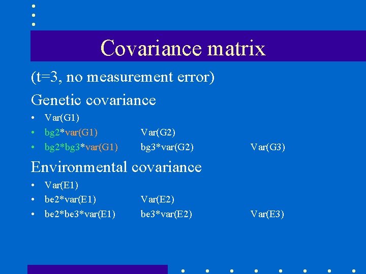
Covariance matrix (t=3, no measurement error) Genetic covariance • Var(G 1) • bg 2*var(G 1) • bg 2*bg 3*var(G 1) Var(G 2) bg 3*var(G 2) Var(G 3) Environmental covariance • Var(E 1) • be 2*var(E 1) • be 2*be 3*var(E 1) Var(E 2) be 3*var(E 2) Var(E 3)

To Mx! • in baalsimplex: 5 datafiles: iq 4[mzm/dzm/mzf/dos]. rec • 8 variables (missing = -1) – t 1 iq 5 t 1 iq 7 t 1 iq 10 t 1 iq 12 t 2 iq 5 t 2 iq 7 t 2 iq 10 t 2 iq 12 • Mx job: guess. mx: incomplete! – For ages 5, 7 and 10 years only – Full of “mistakes” – fix, run for 3 ages, then adjust and run for 4 ages.

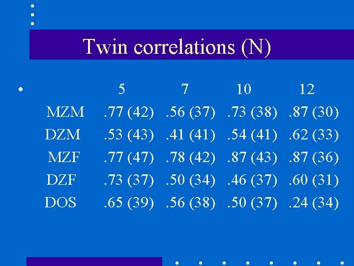
Twin correlations (N) • MZM DZM MZF DOS 5. 77 (42). 53 (43). 77 (47). 73 (37). 65 (39) 7. 56 (37). 41 (41). 78 (42). 50 (34). 56 (38) 10. 73 (38). 54 (41). 87 (43). 46 (37). 50 (37) 12. 87 (30). 62 (33). 87 (36). 60 (31). 24 (34)

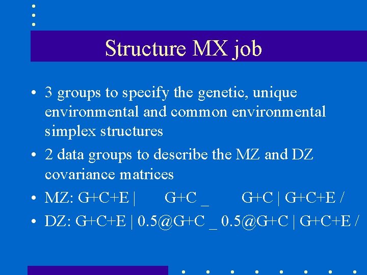
Structure MX job • 3 groups to specify the genetic, unique environmental and common environmental simplex structures • 2 data groups to describe the MZ and DZ covariance matrices • MZ: G+C+E | G+C _ G+C | G+C+E / • DZ: G+C+E | 0. 5@G+C _ 0. 5@G+C | G+C+E /