Developmental Models in Genetic Research David M Evans

Developmental Models in Genetic Research David M. Evans Wellcome Trust Centre for Human Genetics Oxford United Kingdom Sarah E. Medland Queensland Institute of Medical Research Brisbane Australia Twin Workshop Boulder 2004

• These type of models are appropriate whenever one has repeated measures data – short term: trials of an experiment – long term: longitudinal studies • When we have data from genetically informative individuals (e. g. MZ and DZ twins) it is possible to investigate the genetic and environmental influences affecting the trait over time.

What sorts of questions? • Are there changes in the magnitude of genetic and environmental effects over time? • Do the same genetic and environmental influences operate throughout time? • If there are no cohort effects then we can answer the first question using a cross-sectional study type design • However, to answer the second question, longitudinal data is required

“Simplex” Structure From Fischbein (1977) Weight 1 Weight 2 Weight 3 Weight 4 Weight 5 Weight 6 Weight 1 1. 000 Weight 2 0. 985 1. 000 Weight 3 0. 968 0. 981 1. 000 Weight 4 0. 957 0. 970 0. 985 1. 000 Weight 5 0. 932 0. 940 0. 964 0. 975 1. 000 Weight 6 0. 890 0. 897 0. 927 0. 949 0. 973 1. 000

A 1 Y 2 Y 3 Y 4 • “Factor” models tend to fit this type of data poorly (Boomsma & Molenaar, 1987) • => need a type of model which explicitly takes into account the longitudinal nature of the data

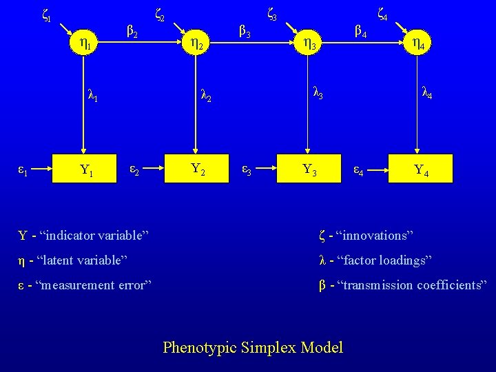
ζ 1 η 1 β 2 Y 1 η 2 β 3 ε 2 Y 2 ζ 3 β 4 η 3 ζ 4 η 4 λ 3 λ 2 λ 1 ε 1 ζ 2 ε 3 λ 4 ε 4 Y 3 Y 4 Y - “indicator variable” ζ - “innovations” η - “latent variable” λ - “factor loadings” ε - “measurement error” β - “transmission coefficients” Phenotypic Simplex Model

ζ 1 η 1 β 2 Y 1 η 2 β 3 ε 2 Y 2 ζ 3 η 3 β 4 ζ 4 λ 3 λ 2 λ 1 ε 1 ζ 2 ε 3 Measurement Model: Y 3 η 4 λ 4 ε 4 Yi = λ i η i + ε i Latent Variable Model: ηi = βi ηi-1 + ζi Y 4

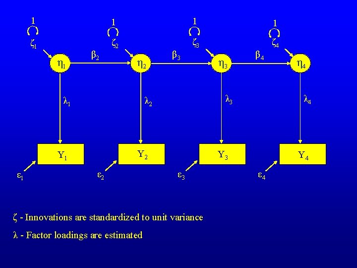
1 1 ζ 1 ζ 2 ζ 3 ζ 4 η 1 β 2 η 2 Y 1 ε 2 ε 3 η 4 λ 4 Y 3 ζ - Innovations are standardized to unit variance λ - Factor loadings are estimated η 3 β 4 λ 3 λ 2 λ 1 ε 1 β 3 Y 4 ε 4

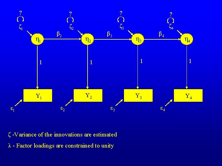
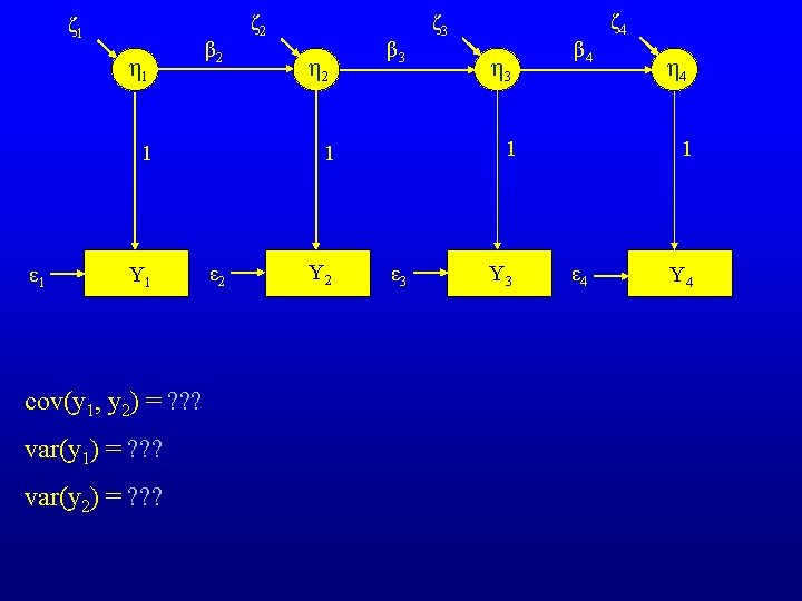
? ? ζ 1 ζ 2 ζ 3 ζ 4 η 1 ε 1 β 2 η 2 β 3 η 3 β 4 η 4 1 1 Y 1 Y 2 Y 3 Y 4 ε 2 ε 3 ζ -Variance of the innovations are estimated λ - Factor loadings are constrained to unity ε 4

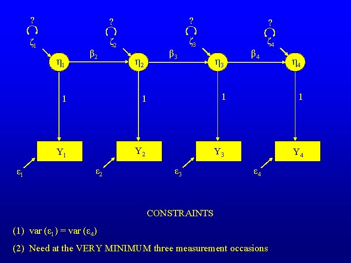
? ? ζ 1 ζ 2 ζ 3 ζ 4 η 1 ε 1 β 2 β 3 η 2 η 3 β 4 η 4 1 1 Y 1 Y 2 Y 3 Y 4 ε 2 ε 3 ε 4 CONSTRAINTS (1) var (ε 1) = var (ε 4) (2) Need at the VERY MINIMUM three measurement occasions

Deriving the Expected Covariance Matrix Path Analysis Matrix Algebra Covariance Algebra

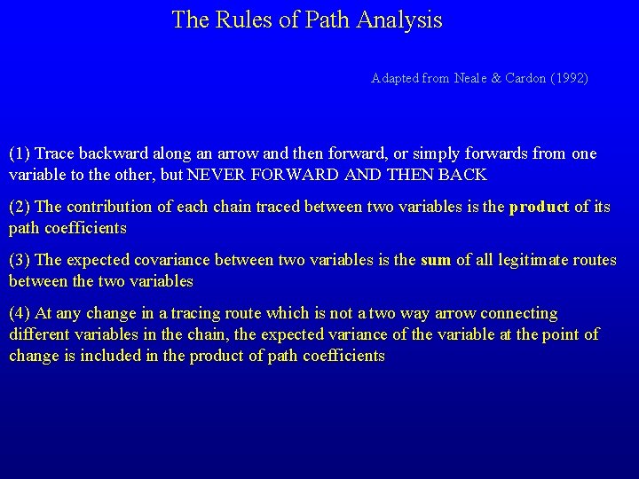
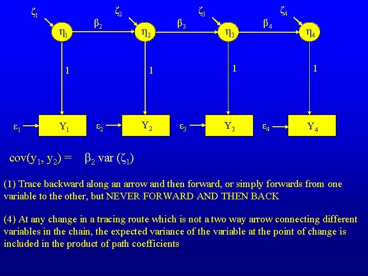
The Rules of Path Analysis Adapted from Neale & Cardon (1992) (1) Trace backward along an arrow and then forward, or simply forwards from one variable to the other, but NEVER FORWARD AND THEN BACK (2) The contribution of each chain traced between two variables is the product of its path coefficients (3) The expected covariance between two variables is the sum of all legitimate routes between the two variables (4) At any change in a tracing route which is not a two way arrow connecting different variables in the chain, the expected variance of the variable at the point of change is included in the product of path coefficients

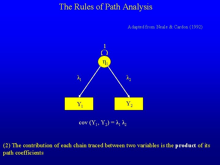
The Rules of Path Analysis Adapted from Neale & Cardon (1992) 1 η 1 λ 2 Y 1 Y 2 cov (Y 1, Y 2) = λ 1 λ 2 (2) The contribution of each chain traced between two variables is the product of its path coefficients

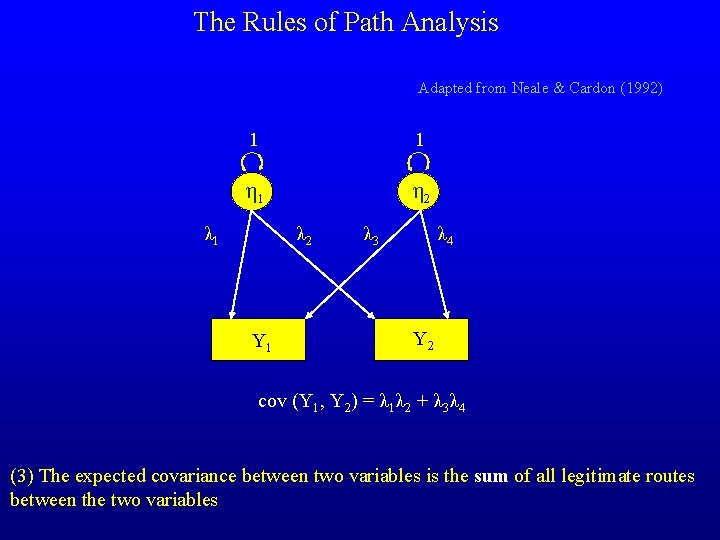
The Rules of Path Analysis Adapted from Neale & Cardon (1992) 1 1 η 2 λ 1 λ 2 Y 1 λ 3 λ 4 Y 2 cov (Y 1, Y 2) = λ 1λ 2 + λ 3λ 4 (3) The expected covariance between two variables is the sum of all legitimate routes between the two variables

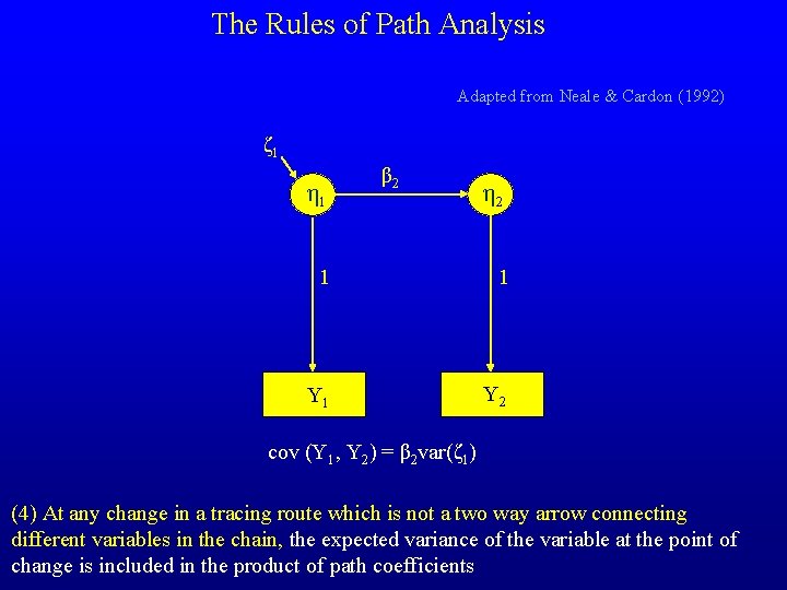
The Rules of Path Analysis Adapted from Neale & Cardon (1992) ζ 1 η 1 β 2 η 2 1 1 Y 2 cov (Y 1, Y 2) = β 2 var(ζ 1) (4) At any change in a tracing route which is not a two way arrow connecting different variables in the chain, the expected variance of the variable at the point of change is included in the product of path coefficients

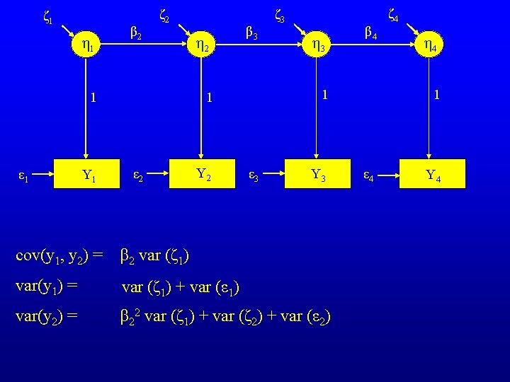
ζ 1 η 1 β 2 ζ 2 Y 1 cov(y 1, y 2) = ε 2 Y 2 η 3 β 4 1 1 1 ε 1 η 2 β 3 ζ 3 ε 3 Y 3 ζ 4 η 4 1 ε 4 Y 4 β 2 var (ζ 1) (1) Trace backward along an arrow and then forward, or simply forwards from one variable to the other, but NEVER FORWARD AND THEN BACK (4) At any change in a tracing route which is not a two way arrow connecting different variables in the chain, the expected variance of the variable at the point of change is included in the product of path coefficients

ζ 1 η 1 β 2 ζ 2 Y 1 ε 2 Y 2 η 3 β 4 1 1 1 ε 1 η 2 β 3 ζ 3 ε 3 Y 3 cov(y 1, y 2) = β 2 var (ζ 1) var(y 1) = var (ζ 1) + var (ε 1) var(y 2) = β 22 var (ζ 1) + var (ζ 2) + var (ε 2) ζ 4 η 4 1 ε 4 Y 4

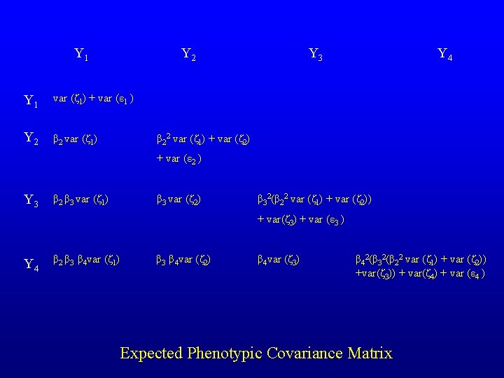
Y 1 Y 2 Y 1 var (ζ 1) + var (ε 1 ) Y 2 β 2 var (ζ 1) Y 3 Y 4 β 22 var (ζ 1) + var (ζ 2) + var (ε 2 ) Y 3 β 2 β 3 var (ζ 1) β 3 var (ζ 2) β 32(β 22 var (ζ 1) + var (ζ 2)) + var(ζ 3) + var (ε 3 ) Y 4 β 2 β 3 β 4 var (ζ 1) β 3 β 4 var (ζ 2) β 4 var (ζ 3) β 42(β 32(β 22 var (ζ 1) + var (ζ 2)) +var(ζ 3)) + var(ζ 4) + var (ε 4 ) Expected Phenotypic Covariance Matrix

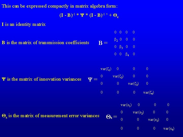
This can be expressed compactly in matrix algebra form: (I - B)-1 * Ψ * (I - B)-1 ’ + Θε I is an identity matrix B is the matrix of transmission coefficients B= 0 0 β 2 0 0 β 3 0 0 var(ζ 1) Ψ is the matrix of innovation variances Ψ= β 4 0 0 0 var(ζ 2) 0 0 var(ζ 3) 0 0 var(ε 1) Θε is the matrix of measurement error variances Θε = var(ζ 4) 0 0 var(ε 2) 0 0 var(ε 3) 0 0 var(ε 4)

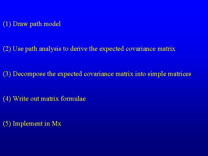
(1) Draw path model (2) Use path analysis to derive the expected covariance matrix (3) Decompose the expected covariance matrix into simple matrices (4) Write out matrix formulae (5) Implement in Mx

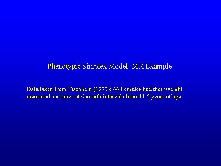
Phenotypic Simplex Model: MX Example Data taken from Fischbein (1977): 66 Females had their weight measured six times at 6 month intervals from 11. 5 years of age.

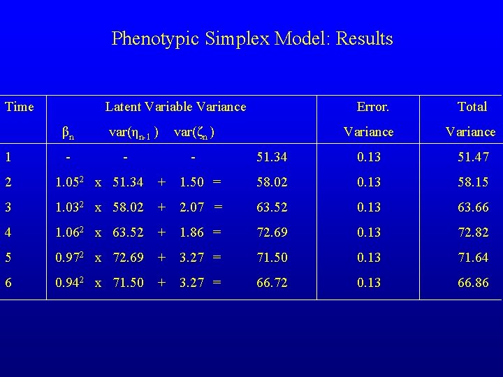
Phenotypic Simplex Model: Results Time Latent Variable Variance βn 1 - var(ηn-1 ) - Error. var(ζn ) - Total Variance 51. 34 0. 13 51. 47 2 1. 052 x 51. 34 + 1. 50 = 58. 02 0. 13 58. 15 3 1. 032 x 58. 02 + 2. 07 = 63. 52 0. 13 63. 66 4 1. 062 x 63. 52 + 1. 86 = 72. 69 0. 13 72. 82 5 0. 972 x 72. 69 + 3. 27 = 71. 50 0. 13 71. 64 6 0. 942 x 71. 50 + 3. 27 = 66. 72 0. 13 66. 86

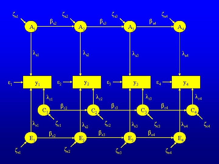
ζa 1 ζa 2 βa 2 A 1 ε 1 βc 2 C 1 E 1 ζe 1 ε 3 ζc 1 βe 2 E 2 ζe 2 ε 4 y 4 λc 3 βc 3 C 2 λe 2 λa 4 y 3 λc 2 λc 1 A 4 λa 3 y 2 ε 2 ζa 4 βa 4 A 3 λa 2 y 1 λe 1 βa 3 A 2 λa 1 ζa 3 ζc 2 E 3 ζe 3 βc 4 C 3 λe 3 βe 3 λc 4 C 4 λe 4 ζc 3 βe 4 E 4 ζe 4 ζc 4

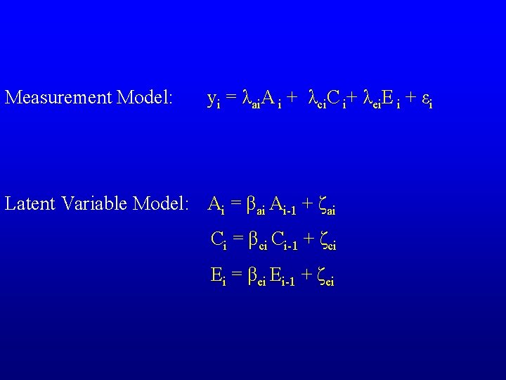
Measurement Model: yi = λai. A i + λci. C i+ λei. E i + εi Latent Variable Model: Ai = βai Ai-1 + ζai Ci = βci Ci-1 + ζci Ei = βei Ei-1 + ζei

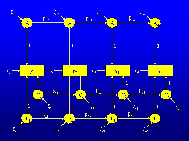
ζa 1 ζa 2 βa 2 A 1 ε 1 βc 2 C 1 E 1 ζe 1 ε 3 ζc 1 βe 2 E 2 ζe 2 ε 4 y 4 1 βc 3 C 2 1 1 y 3 1 1 A 4 1 y 2 ε 2 ζa 4 βa 4 A 3 1 y 1 1 βa 3 A 2 1 ζa 3 ζc 2 E 3 ζe 3 βc 4 C 3 1 βe 3 1 C 4 1 ζc 3 βe 4 E 4 ζe 4 ζc 4

Genetic Simplex Model: MX Example

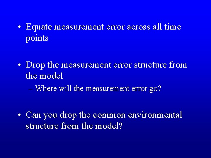
• Equate measurement error across all time points • Drop the measurement error structure from the model – Where will the measurement error go? • Can you drop the common environmental structure from the model?

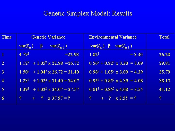
Genetic Simplex Model: Results Time Genetic Variance var(ζn ) 1 4. 792 2 β var(ζn-1 ) =22. 98 Environmental Variance var(ζn ) β var(ζn-1 ) = 3. 30 26. 28 1. 122 + 1. 052 x 22. 98 =26. 72 0. 562 + 0. 922 x 3. 30 = 3. 09 29. 81 3 1. 502 + 1. 042 x 26. 72 = 31. 40 0. 982 + 1. 052 x 3. 09 = 4. 39 35. 79 4 1. 232 + 1. 022 x 31. 40 = 34. 07 0. 952 + 0. 852 x 4. 39 = 4. 08 38. 15 5 1. 392 + 1. 022 x 34. 07 = 37. 57 0. 812 + 0. 852 x 4. 08 = 3. 55 41. 12 6 ? ? ? + ? x 37. 57 = ? 1. 822 Total + ? x 3. 55 = ?

Useful References • Boomsma D. I. & Molenaar P. C. (1987). The genetic analysis of repeated measures. I. Simplex models. Behav Genet, 17(2), 111 -23. • Boomsma D. I. , Martin, N. G. & Molenaar P. C. (1989). Factor and simplex models for repeated measures: application to two psychomotor measures of alcohol sensitivity in twins. Behav Genet, 19(1), 79 -96.

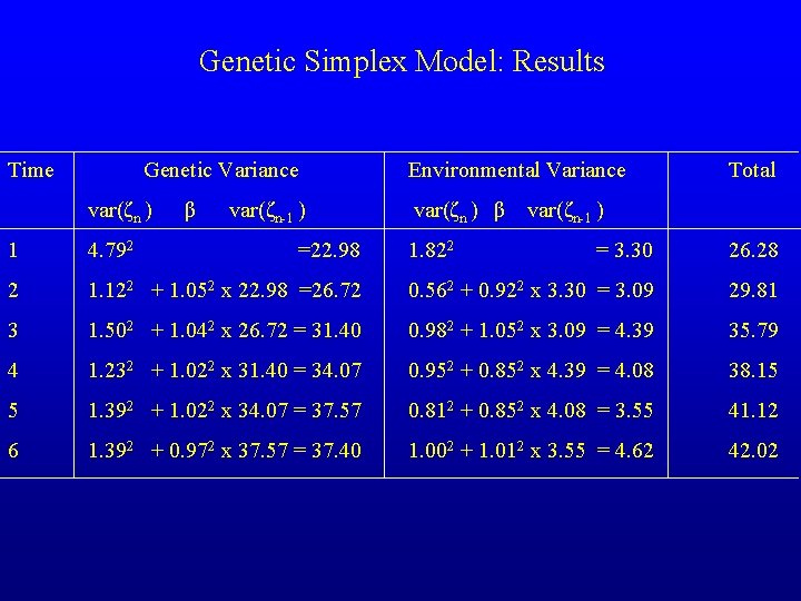
Genetic Simplex Model: Results Time Genetic Variance var(ζn ) 1 4. 792 2 β var(ζn-1 ) =22. 98 Environmental Variance var(ζn ) β 1. 822 Total var(ζn-1 ) = 3. 30 26. 28 1. 122 + 1. 052 x 22. 98 =26. 72 0. 562 + 0. 922 x 3. 30 = 3. 09 29. 81 3 1. 502 + 1. 042 x 26. 72 = 31. 40 0. 982 + 1. 052 x 3. 09 = 4. 39 35. 79 4 1. 232 + 1. 022 x 31. 40 = 34. 07 0. 952 + 0. 852 x 4. 39 = 4. 08 38. 15 5 1. 392 + 1. 022 x 34. 07 = 37. 57 0. 812 + 0. 852 x 4. 08 = 3. 55 41. 12 6 1. 392 + 0. 972 x 37. 57 = 37. 40 1. 002 + 1. 012 x 3. 55 = 4. 62 42. 02