Development of ocean general circulation model to understand

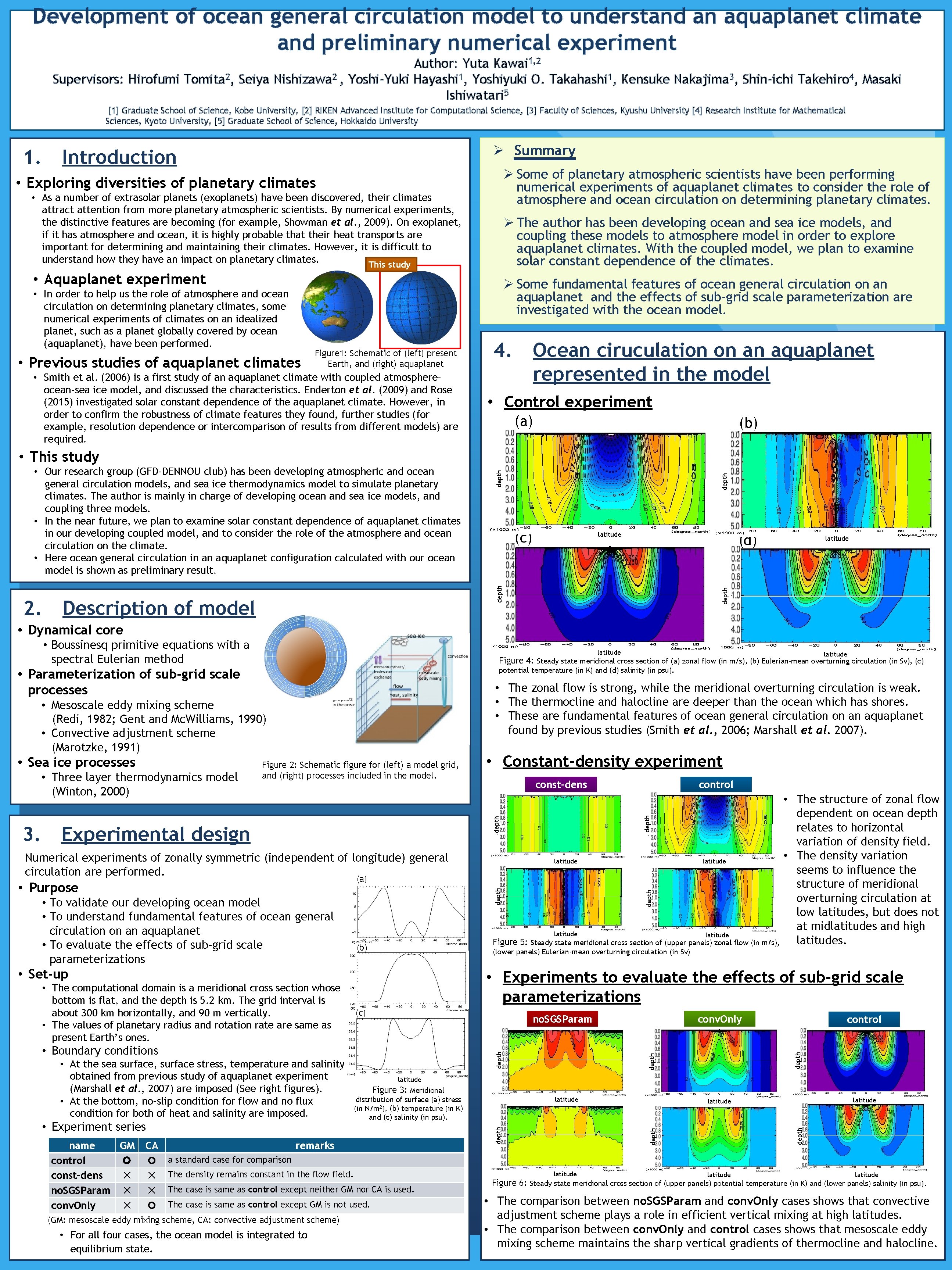
Development of ocean general circulation model to understand an aquaplanet climate and preliminary numerical experiment Author: Yuta Kawai 1, 2 Supervisors: Hirofumi Tomita 2, Seiya Nishizawa 2 , Yoshi-Yuki Hayashi 1, Yoshiyuki O. Takahashi 1, Kensuke Nakajima 3, Shin-ichi Takehiro 4, Masaki Ishiwatari 5 [1] Graduate School of Science, Kobe University, [2] RIKEN Advanced Institute for Computational Science, [3] Faculty of Sciences, Kyushu University [4] Research Institute for Mathematical Sciences, Kyoto University, [5] Graduate School of Science, Hokkaido University 1. Ø Summary Introduction Ø Some of planetary atmospheric scientists have been performing numerical experiments of aquaplanet climates to consider the role of atmosphere and ocean circulation on determining planetary climates. • Exploring diversities of planetary climates • As a number of extrasolar planets (exoplanets) have been discovered, their climates attract attention from more planetary atmospheric scientists. By numerical experiments, the distinctive features are becoming (for example, Showman et al. , 2009). On exoplanet, if it has atmosphere and ocean, it is highly probable that their heat transports are important for determining and maintaining their climates. However, it is difficult to understand how they have an impact on planetary climates. This study Ø The author has been developing ocean and sea ice models, and coupling these models to atmosphere model in order to explore aquaplanet climates. With the coupled model, we plan to examine solar constant dependence of the climates. • Aquaplanet experiment Ø Some fundamental features of ocean general circulation on an aquaplanet and the effects of sub-grid scale parameterization are investigated with the ocean model. • In order to help us the role of atmosphere and ocean circulation on determining planetary climates, some numerical experiments of climates on an idealized planet, such as a planet globally covered by ocean (aquaplanet), have been performed. • Previous studies of aquaplanet climates Figure 1: Schematic of (left) present Earth, and (right) aquaplanet • Smith et al. (2006) is a first study of an aquaplanet climate with coupled atmosphereocean-sea ice model, and discussed the characteristics. Enderton et al. (2009) and Rose (2015) investigated solar constant dependence of the aquaplanet climate. However, in order to confirm the robustness of climate features they found, further studies (for example, resolution dependence or intercomparison of results from different models) are required. 4. Ocean ciruculation on an aquaplanet represented in the model • Control experiment (a) (b) depth latitude (d) Description of model latitude depth 2. (c) depth • Our research group (GFD-DENNOU club) has been developing atmospheric and ocean general circulation models, and sea ice thermodynamics model to simulate planetary climates. The author is mainly in charge of developing ocean and sea ice models, and coupling three models. • In the near future, we plan to examine solar constant dependence of aquaplanet climates in our developing coupled model, and to consider the role of the atmosphere and ocean circulation on the climate. • Here ocean general circulation in an aquaplanet configuration calculated with our ocean model is shown as preliminary result. depth • This study • Dynamical core • Boussinesq primitive equations with a spectral Eulerian method latitude Figure 4: Steady state meridional cross section of (a) zonal flow (in m/s), (b) Eulerian-mean overturning circulation (in Sv), (c) potential temperature (in K) and (d) salinity (in psu). • Parameterization of sub-grid scale processes • The zonal flow is strong, while the meridional overturning circulation is weak. • The thermocline and halocline are deeper than the ocean which has shores. • These are fundamental features of ocean general circulation on an aquaplanet found by previous studies (Smith et al. , 2006; Marshall et al. 2007). Experimental design Numerical experiments of zonally symmetric (independent of longitude) general circulation are performed. (b) (lower panels) Eulerian-mean overturning circulation (in Sv) • Set-up • Experiments to evaluate the effects of sub-grid scale parameterizations no. SGSParam CA ✕ ✕ control latitude Figure 3: Meridional distribution of surface (a) stress (in N/m 2), (b) temperature (in K) and (c) salinity (in psu). remarks latitude depth • Experiment series depth • At the sea surface, surface stress, temperature and salinity obtained from previous study of aquaplanet experiment (Marshall et al. , 2007) are imposed (See right figures). • At the bottom, no-slip condition for flow and no flux condition for both of heat and salinity are imposed. depth • Boundary conditions conv. Only depth (c) depth • The computational domain is a meridional cross section whose bottom is flat, and the depth is 5. 2 km. The grid interval is about 300 km horizontally, and 90 m vertically. • The values of planetary radius and rotation rate are same as present Earth’s ones. depth • To validate our developing ocean model • To understand fundamental features of ocean general circulation on an aquaplanet • To evaluate the effects of sub-grid scale parameterizations control • The structure of zonal flow dependent on ocean depth relates to horizontal variation of density field. • The density variation latitude seems to influence the structure of meridional overturning circulation at low latitudes, but does not at midlatitudes and high latitudes. Figure 5: Steady state meridional cross section of (upper panels) zonal flow (in m/s), depth (a) • Purpose name GM control const-dens ✕ no. SGSParam ✕ conv. Only ✕ const-dens depth 3. • Constant-density experiment depth • Three layer thermodynamics model (Winton, 2000) Figure 2: Schematic figure for (left) a model grid, and (right) processes included in the model. depth • Mesoscale eddy mixing scheme (Redi, 1982; Gent and Mc. Williams, 1990) • Convective adjustment scheme (Marotzke, 1991) • Sea ice processes latitude a standard case for comparison The density remains constant in the flow field. The case is same as control except neither GM nor CA is used. The case is same as control except GM is not used. (GM: mesoscale eddy mixing scheme, CA: convective adjustment scheme) • For all four cases, the ocean model is integrated to equilibrium state. latitude Figure 6: Steady state meridional cross section of (upper panels) potential temperature (in K) and (lower panels) salinity (in psu). • The comparison between no. SGSParam and conv. Only cases shows that convective adjustment scheme plays a role in efficient vertical mixing at high latitudes. • The comparison between conv. Only and control cases shows that mesoscale eddy mixing scheme maintains the sharp vertical gradients of thermocline and halocline.