Development of LowNoise Aircraft Engines Anastasios Lyrintzis School

Development of Low-Noise Aircraft Engines Anastasios Lyrintzis School of Aeronautics & Astronautics Purdue University

Acknowledgements • Indiana 21 st Century Research and Technology Fund • Prof. Gregory Blaisdell • Rolls-Royce, Indianapolis (W. Dalton, Shaym Neerarambam) • L. Garrison, C. Wright, A. Uzun, P-T. Lew

Motivation • Airport noise regulations are becoming stricter. • Lobe mixer geometry has an effect on the jet noise that needs to be investigated.

Methodology • 3 -D Large Eddy Simulation for Jet Aeroacoustics • RANS for Forced Mixers • Coupling between LES and RANS solutions • Semi-empirical method for mixer noise

3 -D Large Eddy Simulation for Jet Aeroacoustics

Objective • Development and full validation of a Computational Aeroacoustics (CAA) methodology for jet noise prediction using: § A 3 -D LES code working on generalized curvilinear grids that provides time-accurate unsteady flow field data § A surface integral acoustics method using LES data for far-field noise computations

Numerical Methods for LES • 3 -D Navier-Stokes equations • 6 th-order accurate compact differencing scheme for spatial derivatives • 6 th-order spatial filtering for eliminating instabilities from unresolved scales and mesh non-uniformities • 4 th-order Runge-Kutta time integration • Localized dynamic Smagorinsky subgrid-scale (SGS) model for unresolved scales

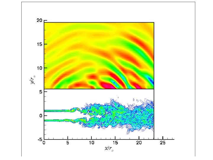
Computational Jet Noise Research • Some of the biggest jet noise computations: § Freund’s DNS for Re. D = 3600, Mach 0. 9 cold jet using 25. 6 million grid points (1999) § Bogey and Bailly’s LES for Re. D = 400, 000, Mach 0. 9 isothermal jets using 12. 5 and 16. 6 million grid points (2002, 2003) • We studied a Mach 0. 9 turbulent isothermal round jet at a Reynolds number of 100, 000 • 12 million grid points used in our LES

Computation Details • Physical domain length of 60 ro in streamwise direction • Domain width and height are 40 ro • 470 x 160 (12 million) grid points • Coarsest grid resolution: 170 times the local Kolmogorov length scale • One month of run time on an IBM-SP using 160 processors to run 170, 000 time steps • Can do the same simulation on the Compaq Alphaserver Cluster at Pittsburgh Supercomputing Center in 10 days

Mean Flow Results • Our mean flow results are compared with: § Experiments of Zaman for initially compressible jets (1998) § Experiment of Hussein et al. (1994) Incompressible round jet at Re. D = 95, 500 § Experiment of Panchapakesan et al. (1993) Incompressible round jet at Re. D = 11, 000

Jet Aeroacoustics • Noise sources located at the end of potential core • Far field noise is estimated by coupling near field LES data with the Ffowcs Williams–Hawkings (FWH) method • Overall sound pressure level values are computed along an arc located at 60 ro from the jet nozzle • Both near and far field acoustic pressure spectra are computed • Assuming at least 6 grid points are required per wavelength, cut-off Strouhal number is around 1. 0

Jet Aeroacoustics (continued) • OASPL results are compared with: § Experiment of Mollo-Christensen et al. (1964) Mach 0. 9 round jet at Re. D = 540, 000 (cold jet) § Experiment of Lush (1971) Mach 0. 88 round jet at Re. D = 500, 000 (cold jet) § Experiment of Stromberg et al. (1980) Mach 0. 9 round jet at Re. D =3, 600 (cold jet) § SAE ARP 876 C database • Acoustic pressure spectra are compared with Bogey and Bailly’s Re. D = 400, 000 isothermal jet

Conclusions • Localized dynamic SGS model very stable and robust for the jet flows we are studying • Very good comparison of mean flow results with experiments • Aeroacoustics results are encouraging • Valuable evidence towards the full validation of our CAA methodology has been obtained

Near Future Work • Simulate Bogey and Bailly’s Re. D = 400, 000 jet test case using 16 million grid points § 100, 000 time steps to run § About 150 hours of run time on the Pittsburgh cluster using 200 processors • Compare results with those of Bogey and Bailly to fully validate CAA methodology • Do a more detailed study of surface integral acoustics methods

Can a realistic LES be done for Re. D = 1, 000 ? • Assuming 50 million grid points provide sufficient resolution: • 200, 000 time steps to run • 30 days of computing time on the Pittsburgh cluster using 256 processors • Only 3 days on a near-future computer that is 10 times faster than the Pittsburgh cluster

RANS for Forced Mixers

Objective • Use RANS to study flow characteristics of various flow shapes

What is a Lobe Mixer?

Lobe Penetration

Current Progress • Only been able to obtain a ‘high penetration’ mixer for CFD analysis. • Have completed all of the code and turbulence model comparisons with single mixer.

3 -D Mesh

WIND Code options • • • 2 nd order upwind scheme 1. 7 million/7 million grid points 8 -16 zones 8 -16 LINUX processors Spalart-Allmaras/ SST turbulence model Wall functions

Grid Dependence Density Contours 1. 7 million grid points Density Contours 7 million grid points

Grid Dependence 1. 7 million grid points Density Vorticity Magnitude

Spalart-Allmaras and Menter SST Turbulence Models Spalart-Allmaras Menter SST

Spalart-Allmaras and Menter SST at Nozzle Exit Plane SST Spalart Density Vorticity Magnitude

Turbulence Intensity at x/d =. 4 Menter SST model Experiment, NASA Glenn 1996 WIND

Mean Axial Velocity at x/d =. 4 Spalart-Allmaras Menter SST Experiment, NASA Glenn 1996 WIND

Turbulence Intensity at x/d = 1. 0 Menter SST model Experiment, NASA Glenn 1996 WIND

Mean Axial Velocity at x/d = 1. 0 Spalart-Allmaras Experiment, NASA Glenn 1996 WIND Menter SST WIND

Spalart-Allmaras vs. Menter SST • The Spalart-Allmaras model appears to be less dissipative. The vortex structure is sharper and the vorticity magnitude is higher at the nozzle exit. • The Menter SST model appears to match experiments better, but the experimental grid is rather coarse and some of the finer flow structure may have been effectively filtered out. • Still unclear which model is superior. No need to make a firm decision until several additional geometries are obtained.

Preliminary Conclusions • 1. 7 million grid is adequate • Further work is needed comparing the turbulence models

Future Work • Analyze the flow fields and compare to experimental acoustic and flow-field data for additional mixer geometries. • Further compare the two turbulence models. • If possible, develop qualitative relationship between mean flow characteristics and acoustic performance.

Implementing RANS Inflow Boundary Conditions for 3 -D LES Jet Aeroacoustics

Objectives • Implement RANS solution and onto 3 -D LES inflow BCs as initial conditions. • Investigate the effect of RANS inflow conditions on turbulent properties such as: – Reynolds Stresses – Far-field sound generated

Implementation Method LES RANS • RANS grid too fine for LES grid to match. • Since RANS grid has high resolution, linear interpolation will be used.

Issues and Challenges • • • Accurate resolution of outgoing vortex with LES grid. Accurate resolution of shear layer near nozzle lip. May need to use an intermediate Reynolds number eg. Re = 400, 000

An Investigation of Extensions of the Four. Source Method for Predicting the Noise From Jets With Internal Forced Mixers

Four-Source Coaxial Jet Noise Prediction Secondary / Ambient Shear Layer Primary / Secondary Shear Layer Vs Vp Vs Initial Region Interaction Region Mixed Flow Region

Four-Source Coaxial Jet Noise Prediction – Secondary Jet: – Effective Jet: – Mixed Jet: – Total noise is the incoherent sum of the noise from the three jets

Forced Mixer H H: Lobe Penetration (Lobe Height)

Nozzle Internally Forced Mixed Jet Bypass Flow Mixer Exhaust Flow Core Flow Tail Cone Lobed Mixer Mixing Layer Exhaust / Ambient Mixing Layer

Noise Prediction Comparisons • Experimental Data – Aeroacoustic Propulsion Laboratory at NASA Glenn – Far-field acoustic measurements (~80 diameters) • Single Jet Prediction – Based on nozzle exhaust properties (V, T, D) – SAE ARP 876 C • Coaxial Jet Prediction – Four-source method – SAE ARP 876 C for single jet predictions

Noise Prediction Comparisons Low Penetration Mixer High Penetration Mixer

Noise Prediction Comparisons Low Penetration Mixer High Penetration Mixer

Noise Prediction Comparisons Low Penetration Mixer High Penetration Mixer

Modified Four-Source Formulation Single Jet Prediction Variable Parameters: Spectral Filter Source Reduction

Modified Formulation Variable Parameters Dd. B Dfc

Parameter Optimization Algorithm • Frequency range is divided into three sub-domains • Start with uncorrected single jet sources • Evaluate the error in each frequency sub-domain and adjusted relevant parameters • Iterate until a solution is converged upon Low Frequency Sub -Domain Mid Frequency -Domain Sub High Frequency Sub-Domain Dd. Bm , Dd. Be Dd. Bs , Dd. Bm , Dd. Be Dd. Bs fs fs , fm , fe

Parameter Optimization Algorithm Low Frequency Sub. Mid Frequency Sub High Frequency -Domain Sub-Domain

Parameter Optimization Results Low Penetration Mixer High Penetration Mixer

Modified Method with Optimized Parameters Low Penetration Mixer High Penetration Mixer

Modified Method with Optimized Parameters Low Penetration Mixer High Penetration Mixer

Modified Method with Optimized Parameters Low Penetration Mixer High Penetration Mixer

Optimized Parameter Trends • Dd. Bs (Increased) – Influenced by the convergent nozzle and mixing of the secondary flow with the faster primary flow – The exhaust jet velocity will be greater than the secondary jet velocity resulting in a noise increase

Optimized Parameter Trends • Dd. Bm (Decreased) – Influenced by the effect of the interactions of the mixing layer generated by the mixer with the outer ambientexhaust shear layer – The mixer effects cause the fully mixed jet to diffuse faster resulting in a larger effective diameter and therefore a lower velocity, resulting in a noise reduction

Optimized Parameter Trends • fc (Increased) – Influenced by the location where the turbulent mixing layer generated by the lobe mixer intersects the ambientexhaust shear layer

Summary • In general the coaxial and single jet prediction methods do not accurately model the noise from jets with internal forced mixers • The forced mixer noise spectrum can be matched using the combination of two single jet noise sources • Currently not a predictive method • Next step is to evaluate the optimized parameters for additional mixer data – Additional Mixer Geometries – Additional Flow Conditions (Velocities and Temperatures) • Identify trends and if possible empirical relationships between the mixer geometries and their optimized parameters

Conclusion • Methodologies (LES, RANS, semiempirical method) have been developed to study noise from forced mixers