Development of Empirical Models From Process Data Chapter

Development of Empirical Models From Process Data Chapter 7 • In some situations it is not feasible to develop a theoretical (physically-based model) due to: 1. Lack of information 2. Model complexity 3. Engineering effort required. • An attractive alternative: Develop an empirical dynamic model from input-output data. • Advantage: less effort is required • Disadvantage: the model is only valid (at best) for the range of data used in its development. i. e. , empirical models usually don’t extrapolate very well. 1

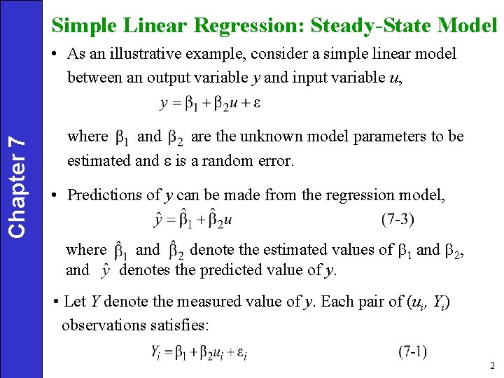
Simple Linear Regression: Steady-State Model Chapter 7 • As an illustrative example, consider a simple linear model between an output variable y and input variable u, where and are the unknown model parameters to be estimated and e is a random error. • Predictions of y can be made from the regression model, where and denote the estimated values of b 1 and b 2, and denotes the predicted value of y. • Let Y denote the measured value of y. Each pair of (ui, Yi) observations satisfies: 2

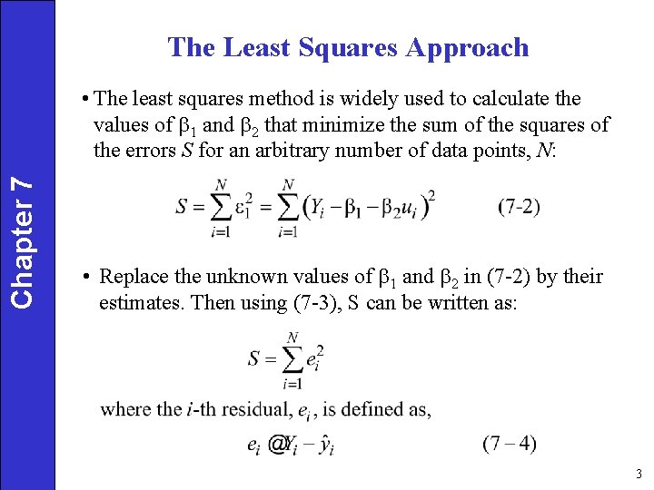
The Least Squares Approach Chapter 7 • The least squares method is widely used to calculate the values of b 1 and b 2 that minimize the sum of the squares of the errors S for an arbitrary number of data points, N: • Replace the unknown values of b 1 and b 2 in (7 -2) by their estimates. Then using (7 -3), S can be written as: 3

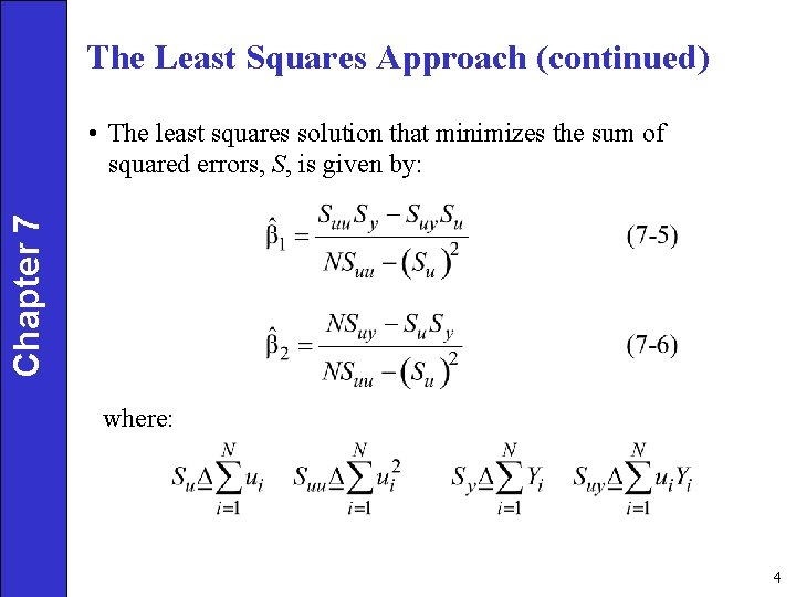
The Least Squares Approach (continued) Chapter 7 • The least squares solution that minimizes the sum of squared errors, S, is given by: where: 4

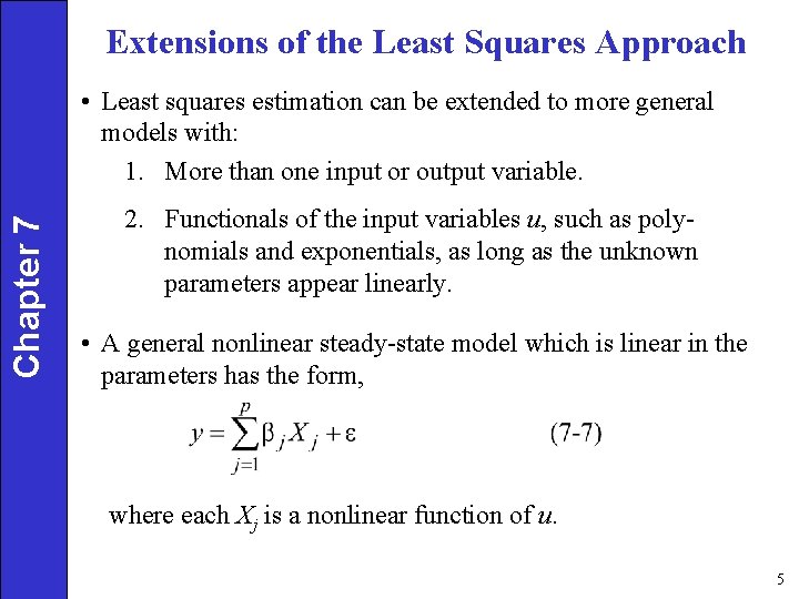
Extensions of the Least Squares Approach Chapter 7 • Least squares estimation can be extended to more general models with: 1. More than one input or output variable. 2. Functionals of the input variables u, such as polynomials and exponentials, as long as the unknown parameters appear linearly. • A general nonlinear steady-state model which is linear in the parameters has the form, where each Xj is a nonlinear function of u. 5

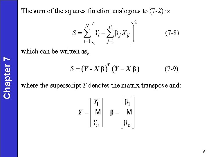
The sum of the squares function analogous to (7 -2) is Chapter 7 which can be written as, where the superscript T denotes the matrix transpose and: 6

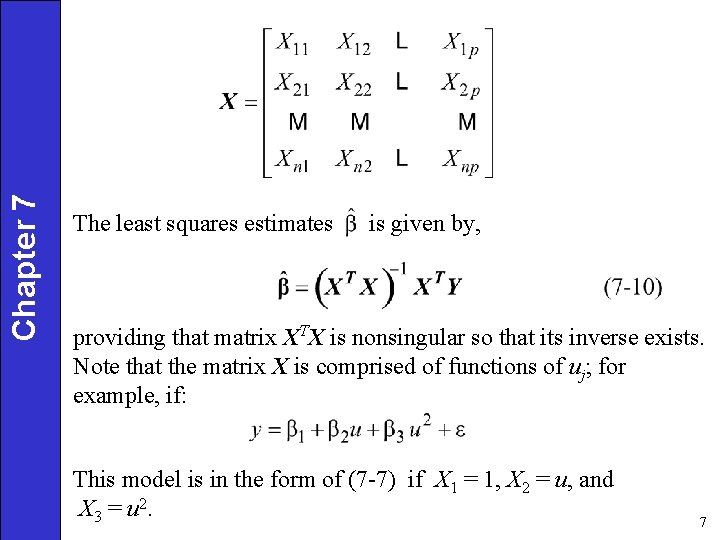
Chapter 7 The least squares estimates is given by, providing that matrix XTX is nonsingular so that its inverse exists. Note that the matrix X is comprised of functions of uj; for example, if: This model is in the form of (7 -7) if X 1 = 1, X 2 = u, and X 3 = u 2. 7

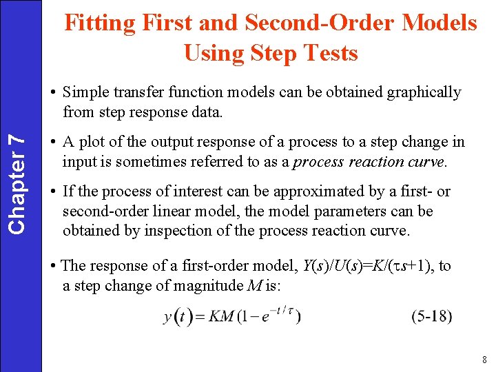
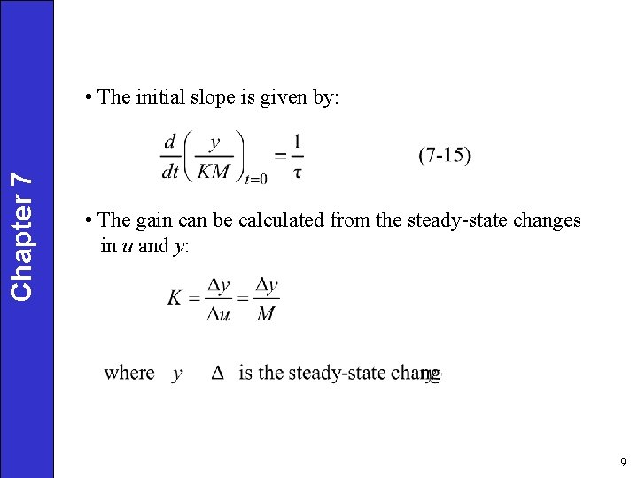
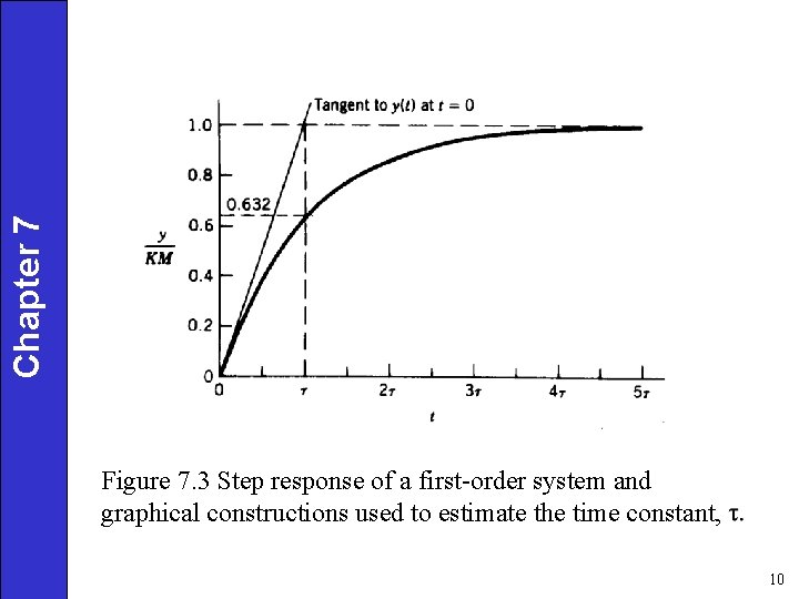
Fitting First and Second-Order Models Using Step Tests Chapter 7 • Simple transfer function models can be obtained graphically from step response data. • A plot of the output response of a process to a step change in input is sometimes referred to as a process reaction curve. • If the process of interest can be approximated by a first- or second-order linear model, the model parameters can be obtained by inspection of the process reaction curve. • The response of a first-order model, Y(s)/U(s)=K/( s+1), to a step change of magnitude M is: 8

Chapter 7 • The initial slope is given by: • The gain can be calculated from the steady-state changes in u and y: 9

Chapter 7 Figure 7. 3 Step response of a first-order system and graphical constructions used to estimate the time constant, 10

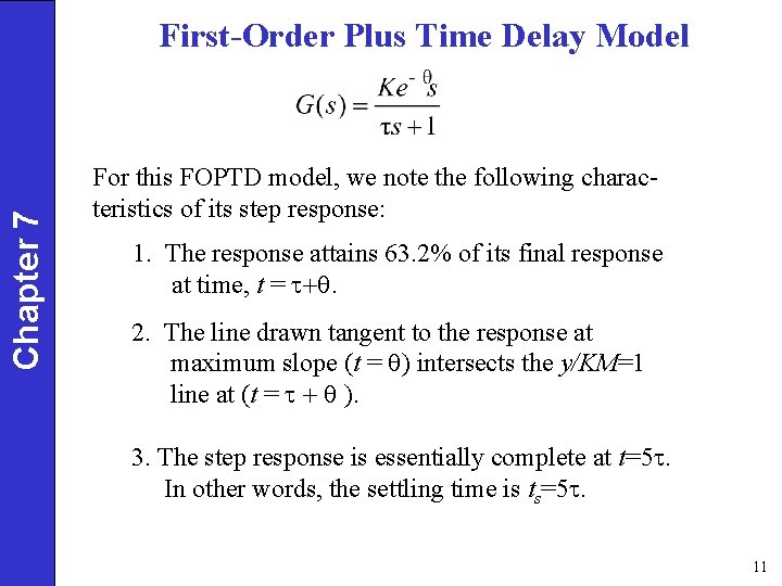
Chapter 7 First-Order Plus Time Delay Model For this FOPTD model, we note the following characteristics of its step response: 1. The response attains 63. 2% of its final response at time, t = . 2. The line drawn tangent to the response at maximum slope (t = ) intersects the y/KM=1 line at (t = ). 3. The step response is essentially complete at t=5. In other words, the settling time is ts=5. 11

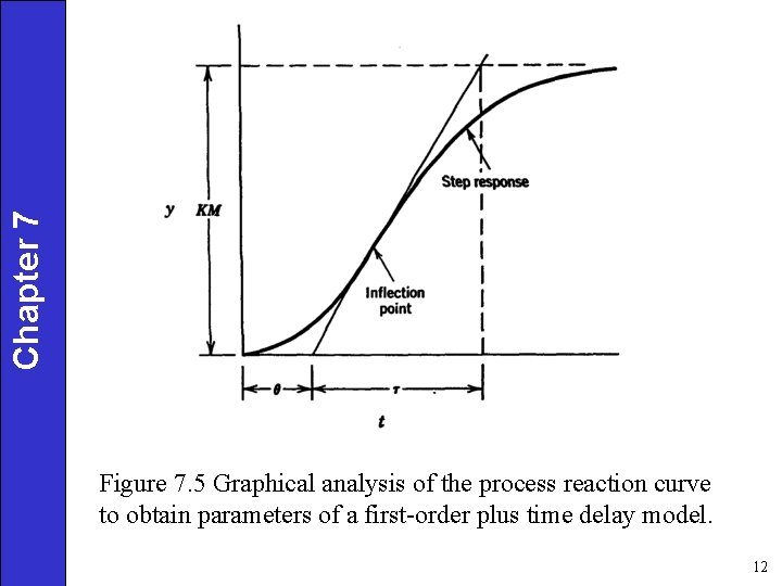
Chapter 7 Figure 7. 5 Graphical analysis of the process reaction curve to obtain parameters of a first-order plus time delay model. 12

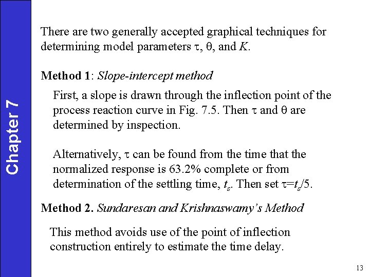
There are two generally accepted graphical techniques for determining model parameters , , and K. Chapter 7 Method 1: Slope-intercept method First, a slope is drawn through the inflection point of the process reaction curve in Fig. 7. 5. Then and are determined by inspection. Alternatively, can be found from the time that the normalized response is 63. 2% complete or from determination of the settling time, ts. Then set =ts/5. Method 2. Sundaresan and Krishnaswamy’s Method This method avoids use of the point of inflection construction entirely to estimate the time delay. 13

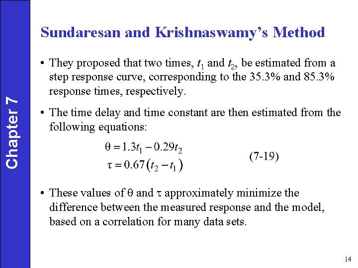
Chapter 7 Sundaresan and Krishnaswamy’s Method • They proposed that two times, t 1 and t 2, be estimated from a step response curve, corresponding to the 35. 3% and 85. 3% response times, respectively. • The time delay and time constant are then estimated from the following equations: • These values of and approximately minimize the difference between the measured response and the model, based on a correlation for many data sets. 14

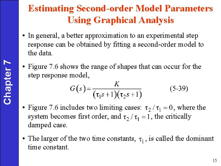
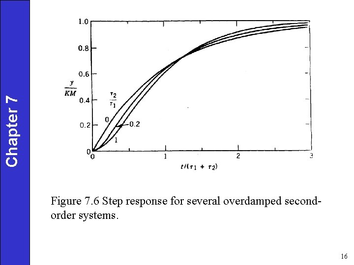
Estimating Second-order Model Parameters Using Graphical Analysis Chapter 7 • In general, a better approximation to an experimental step response can be obtained by fitting a second-order model to the data. • Figure 7. 6 shows the range of shapes that can occur for the step response model, • Figure 7. 6 includes two limiting cases: system becomes first order, and damped case. • The larger of the two time constants, time constant. , where the , the critically , is called the dominant 15

Chapter 7 Figure 7. 6 Step response for several overdamped secondorder systems. 16

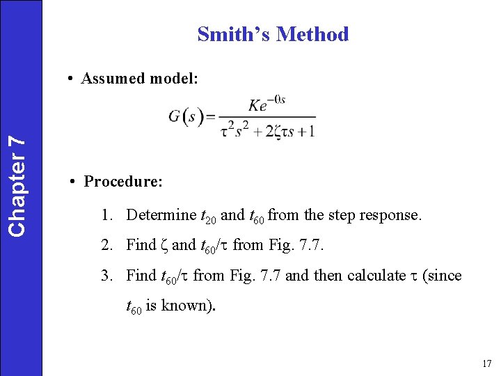
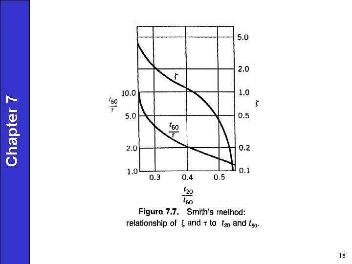
Smith’s Method Chapter 7 • Assumed model: • Procedure: 1. Determine t 20 and t 60 from the step response. 2. Find ζ and t 60/ from Fig. 7. 7. 3. Find t 60/ from Fig. 7. 7 and then calculate (since t 60 is known). 17

18 Chapter 7

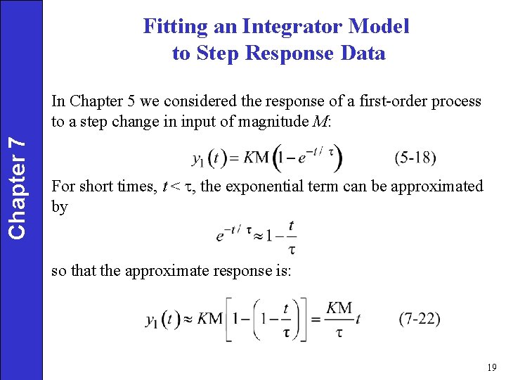
Fitting an Integrator Model to Step Response Data Chapter 7 In Chapter 5 we considered the response of a first-order process to a step change in input of magnitude M: For short times, t < , the exponential term can be approximated by so that the approximate response is: 19

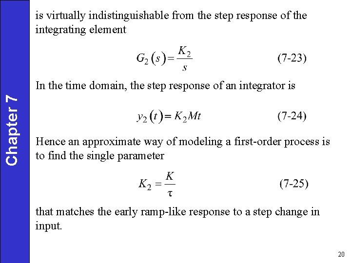
is virtually indistinguishable from the step response of the integrating element Chapter 7 In the time domain, the step response of an integrator is Hence an approximate way of modeling a first-order process is to find the single parameter that matches the early ramp-like response to a step change in input. 20

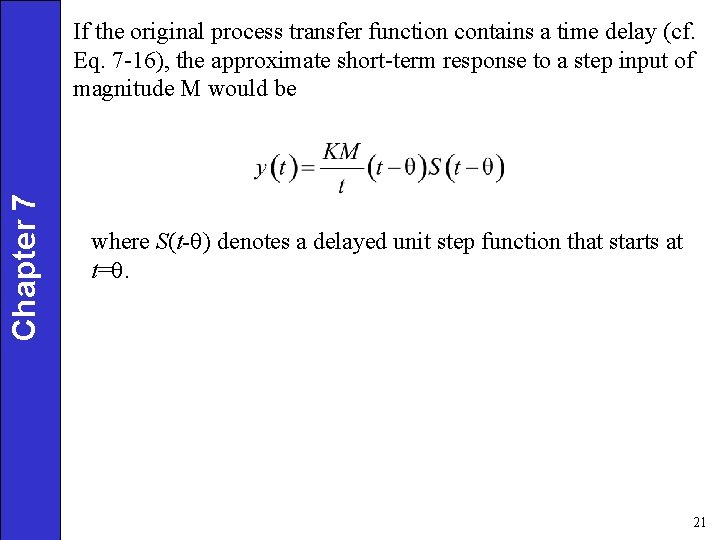
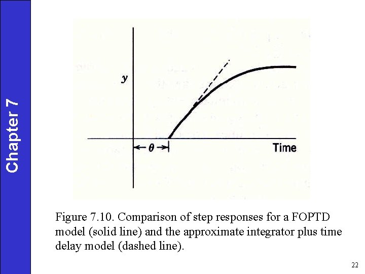
Chapter 7 If the original process transfer function contains a time delay (cf. Eq. 7 -16), the approximate short-term response to a step input of magnitude M would be where S(t- ) denotes a delayed unit step function that starts at t=. 21

Chapter 7 Figure 7. 10. Comparison of step responses for a FOPTD model (solid line) and the approximate integrator plus time delay model (dashed line). 22

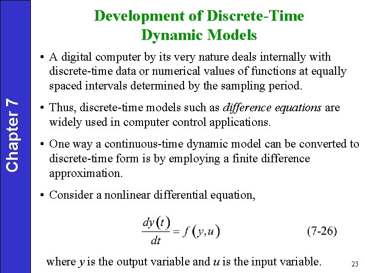
Development of Discrete-Time Dynamic Models Chapter 7 • A digital computer by its very nature deals internally with discrete-time data or numerical values of functions at equally spaced intervals determined by the sampling period. • Thus, discrete-time models such as difference equations are widely used in computer control applications. • One way a continuous-time dynamic model can be converted to discrete-time form is by employing a finite difference approximation. • Consider a nonlinear differential equation, where y is the output variable and u is the input variable. 23

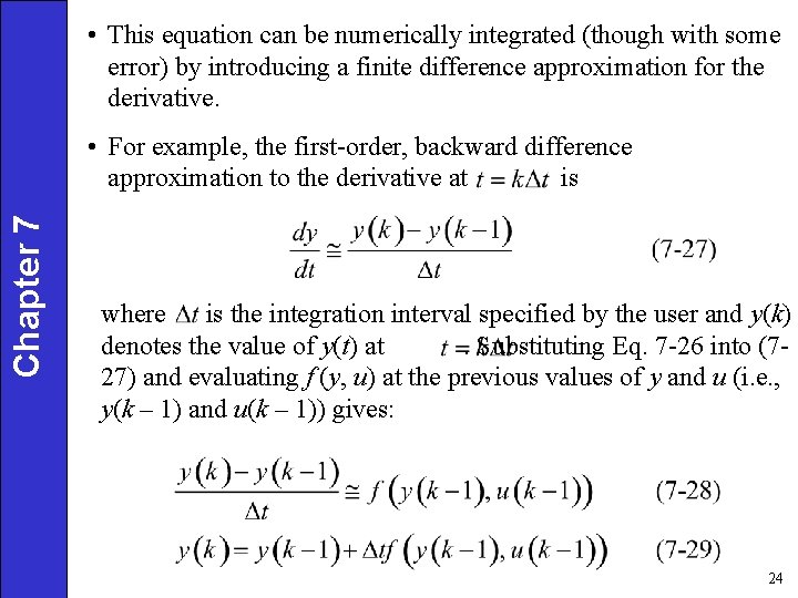
• This equation can be numerically integrated (though with some error) by introducing a finite difference approximation for the derivative. Chapter 7 • For example, the first-order, backward difference approximation to the derivative at is where is the integration interval specified by the user and y(k) denotes the value of y(t) at. Substituting Eq. 7 -26 into (727) and evaluating f (y, u) at the previous values of y and u (i. e. , y(k – 1) and u(k – 1)) gives: 24

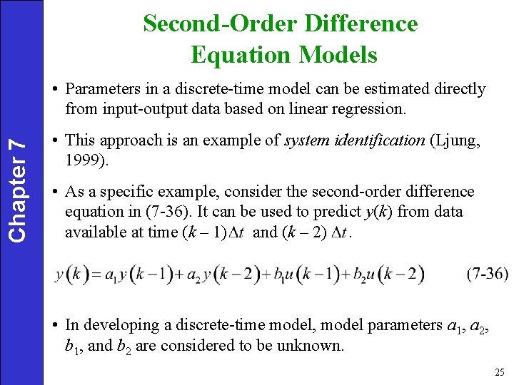
Second-Order Difference Equation Models Chapter 7 • Parameters in a discrete-time model can be estimated directly from input-output data based on linear regression. • This approach is an example of system identification (Ljung, 1999). • As a specific example, consider the second-order difference equation in (7 -36). It can be used to predict y(k) from data available at time (k – 1) and (k – 2). • In developing a discrete-time model, model parameters a 1, a 2, b 1, and b 2 are considered to be unknown. 25

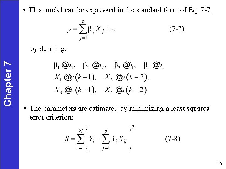
• This model can be expressed in the standard form of Eq. 7 -7, Chapter 7 by defining: • The parameters are estimated by minimizing a least squares error criterion: 26

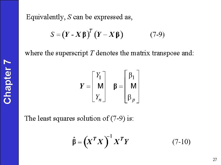
Equivalently, S can be expressed as, Chapter 7 where the superscript T denotes the matrix transpose and: The least squares solution of (7 -9) is: 27