Development Economics ECON 4915 Lecture 5 Andreas Kotsadam

Development Economics ECON 4915 Lecture 5 Andreas Kotsadam

Outline • Seminar 3 • Empirical methods ØRandomisation ØOther methods: IV, DDD, RD. Ø Discussion: Internal vs. External validity. • Possible exam question on insurance and recap from last lecture.

Seminar 3 • Seminar group 1, i. e. the group starting at 12. 15 have choosen: Acemoglu et al. ; Jensen and Oster; Nunn and Wantchekon; Qian. • The after-lunch group have choosen: Beaman et al. ; Jensen and Oster. • Two sub-groups are missing here!!!

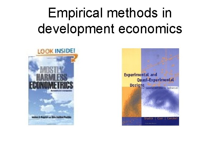
Empirical methods in development economics

Other interesting references • Symposium in The Journal of Economic Perspectives, Volume 24, Number 2, Spring 2010. Starting with: • Angrist and Pischke, “The Credibility Revolution in Empirical Economics: How Better Research Design Is Taking the Con out of Econometrics” • See also: • Deaton (2009) ”Instruments of development: Randomization in the tropics, and the search for the elusive keys to economic development”. • Banarjee and Duflo (2009) ”The experimental approach to development economics”.

The fundamental problem of causal inference • Answering any causal question requires knowing the counterfactual. • At the individual level this is impossible. • Maybe we can solve this by using statistics?

We need a comparison group • . . . that would have had similar outcomes as the treatment group if there was no treatment. • In general, however, those recieving treatment and those that do not usually differ due to: → Targeting → Screening → Self-selection.

This implies • . . . that those not exposed to a treatment are often a lousy comparison group. • It is often impossible to disentangle treatment effects from selection bias.

Example • A fertilizer program where fertilizers are given for free to some farmers.

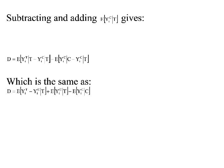
We want to know the effect Effect= Yield for the farmers who got fertilizer Yield at the same point in time for the same farmers in absence of the program.

Problem We never observe the same individual with and without program at the same point in time.

We cannot simply compare before and after • Other things may happen over time so that we cannot separate the effect of the treatment and the effect of those other things. • Even if you know ”nothing else happened” it is hard to convince others. • The burden of proof is on you.

We cannot simply compare with those who did not get fertilizers • Some may choose not to participate. • Those not offered the program may differ. • Again, the burden of proof is on you.

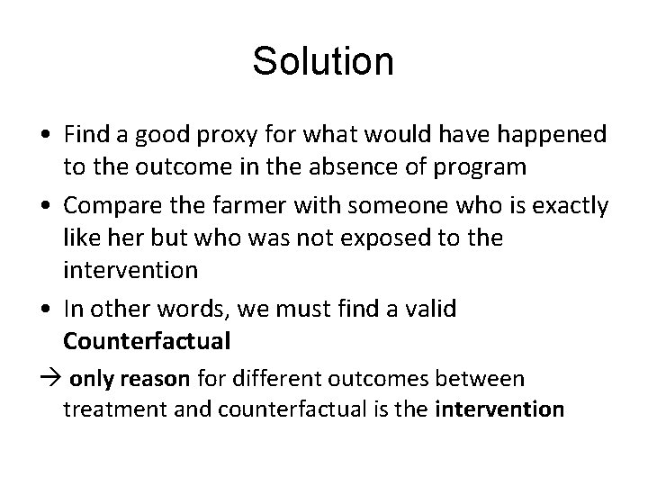
Solution • Find a good proxy for what would have happened to the outcome in the absence of program • Compare the farmer with someone who is exactly like her but who was not exposed to the intervention • In other words, we must find a valid Counterfactual only reason for different outcomes between treatment and counterfactual is the intervention

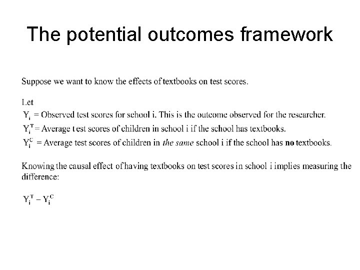
The potential outcomes framework

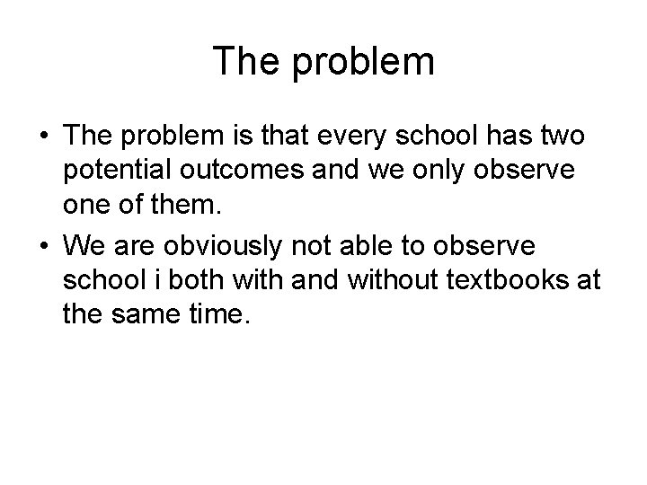
The problem • The problem is that every school has two potential outcomes and we only observe one of them. • We are obviously not able to observe school i both with and without textbooks at the same time.

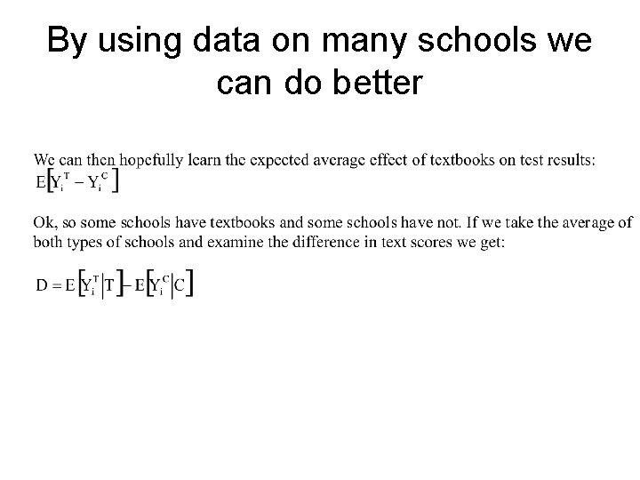
By using data on many schools we can do better

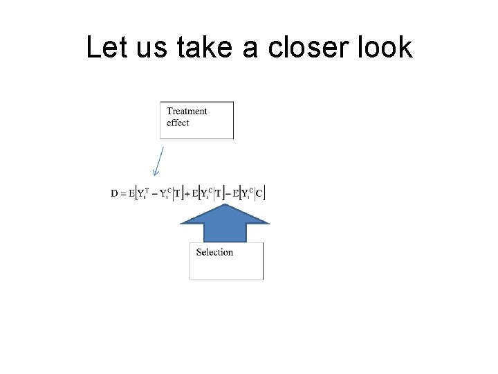
Let us take a closer look

Examples of selection effects in the textbook example: • 1) • 2)

The general point • In addition to the effect of textbooks there may be other systematic differences between schools with and without textbooks. • The goal is to find situations where selection bias does not exist or where we can correct for it.

Randomization • When individuals, or schools, or countries, are randomly assigned to treatment and comparison groups, the selection bias disappears. • Take a sample of N individuals from a population of interest. • Divide the sample randomly into a treatment and a control group.

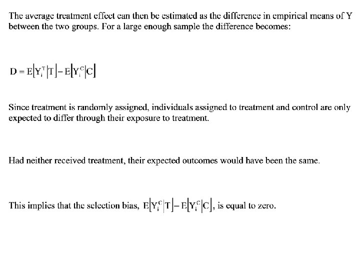
Randomization • Then give the treatment group a treatment so that their treatment status is T and nothing to the control group so that their treatment status is C. • Collect outcome data Y and compare the treatment average to the control average.

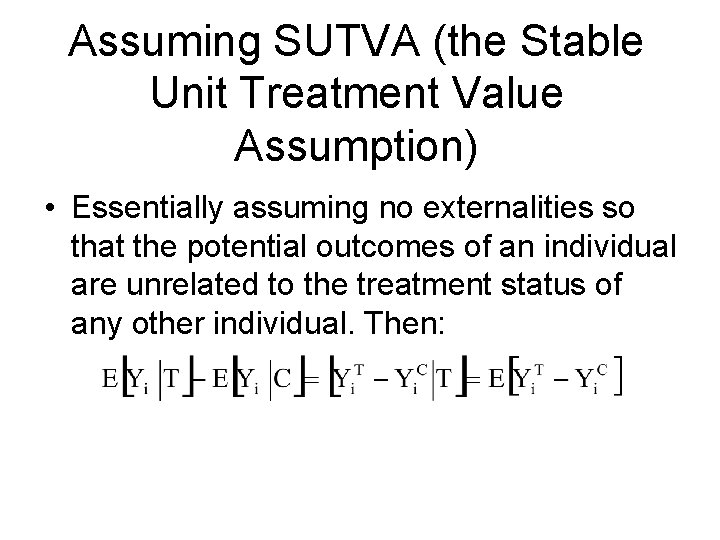
Assuming SUTVA (the Stable Unit Treatment Value Assumption) • Essentially assuming no externalities so that the potential outcomes of an individual are unrelated to the treatment status of any other individual. Then:

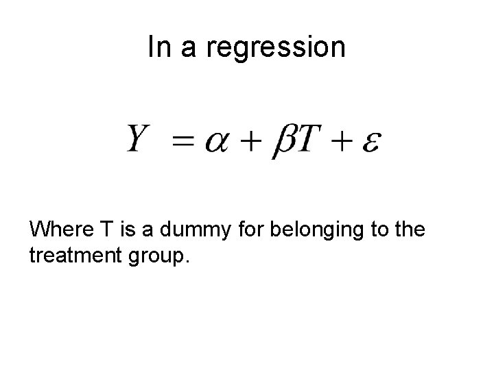
In a regression Where T is a dummy for belonging to the treatment group.

A detour on the law of large numbers • ” For a large enough sample… ” • If we were to draw a line in the middle of India and randomly (e. g. by flipping a coin) provide microcredit in one part this would be a randomized field experiment. • ”Large enough” depends on the variance and magnitude of the effects.

What is being estimated? • We get the overall impact of a particular treatment on an outcome. • Note in particular that we allow other things to change as a response to the program. • It is not the all else equal effect. • ”Reduced form”: Total derivative.

Main advantages of randomization • A randomized evaluation provides internally valid estimates = It provides an unbiased estimate of the impact of the program in the sample under study. • They are also easy to understand. • Very good for testing theories.

Critiques of randomized experiments • External validity: = Is the effect generalizable to other samples? • A) Environmental dependence: Would providing free school lunch have the same effect in Norway and in Kenya? Obviously not, but the trickier question is where to draw the line: Is Argentina more like Norway or Kenya?

External validy continued • B) Implementer effects: The results may not generalize to other NGO’s for example. More problematic, not every NGO wants to be evaluated: Probably a selection of more competent NGOs and better programs!

But these issues apply to all empirical work • Argentina is not more like Norway because we build a model. • Countries with better institutions often have better data.

More critique • General equilibrium effects: What happens if we scale up a successful program? • Randomization bias: The fact that the program is evaluated using randomization affects behavior. • Hawthorne effect: Being monitored changes behavior.

Ethics • Is randomization unfair? • Why so many experiments from developing countries? • Generous interpretation: The questions merit it and there is not a lot of data to work with. • More cynical interpretation: It is cheap and feasible (e. g. no ethical review board).

Why not more randomized impact evaluations? • Ignorance may have political advantages. • Technical capacity may be limited. • Benefits are not clearly appropriated to those who bear the costs: Evaluations as a public good. • And randomization is simply not always feasible.

If randomization is not possible • Other methods can be used to handle selection bias but they all require more assumptions. • These identifying assumptions are not testable and the validity of any particular study depends on how convincing these assumptions appear. • Identification strategy= research design to identify a causal effect.

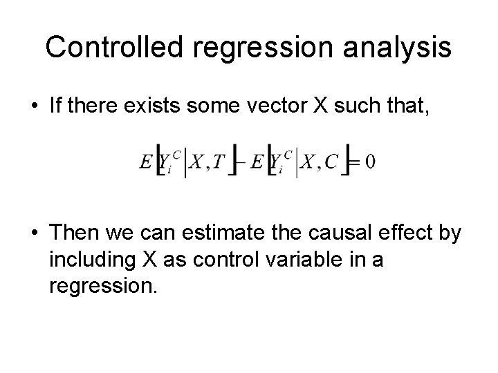
Controlled regression analysis • If there exists some vector X such that, • Then we can estimate the causal effect by including X as control variable in a regression.

Problems • This approach is only valid if there is no difference in potential outcomes between treated and untreated individuals once we have controlled for the observable differences. • It is generally unlikely that this is enough since X must account for all the relevant observed and unobserved differences between the treatment and control groups.

Instrumental variables (IV) • Very common method in empirical economics. • We saw it it B&P in lecture 2 and we will see it in several other papers during the course. • A very good reference for IV is Murray (2006) ”The Bad, the Weak, and the Ugly: Avoiding the Pitfalls of Instrumental Variables Estimation”

Instrumental variables (IV) • What’s the problem? • How can it be solved by IV? • How is it done in practice? Examples. • Instruments can be: i) Bad, ii) Weak, iii) Ugly.

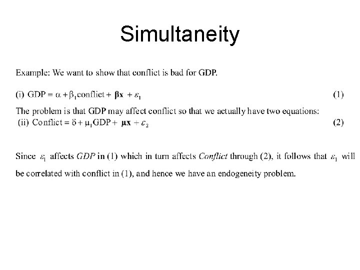
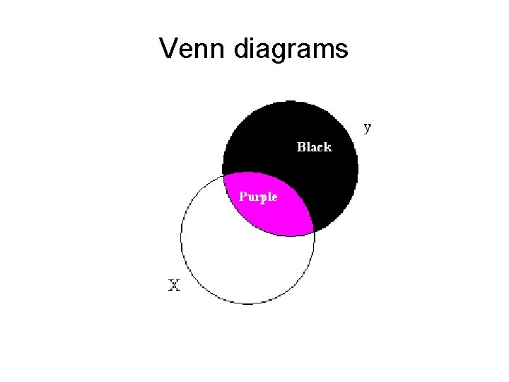
What’s the problem? • IV solves the problem of ”endogeneity”. • Endogeneity: An explanatory variable is correlated with the error term. • Very common in social science. • Most common reasons: i) Omitted variables ii) Measurement error iii) Simultaneity (reversed causation)

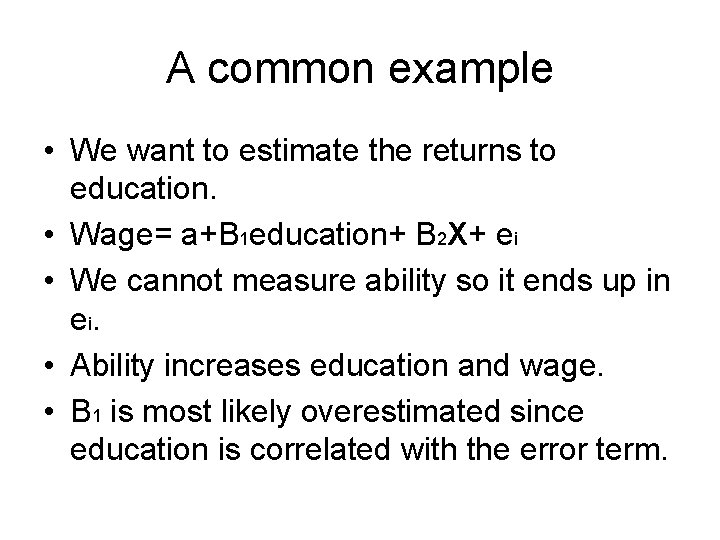
A common example • We want to estimate the returns to education. • Wage= a+B 1 education+ B 2 X+ ei • We cannot measure ability so it ends up in e i. • Ability increases education and wage. • B 1 is most likely overestimated since education is correlated with the error term.

Simultaneity

What can be done? • To overcome the endogeneity problem we can use the Instrumental Variables (IV) approach.

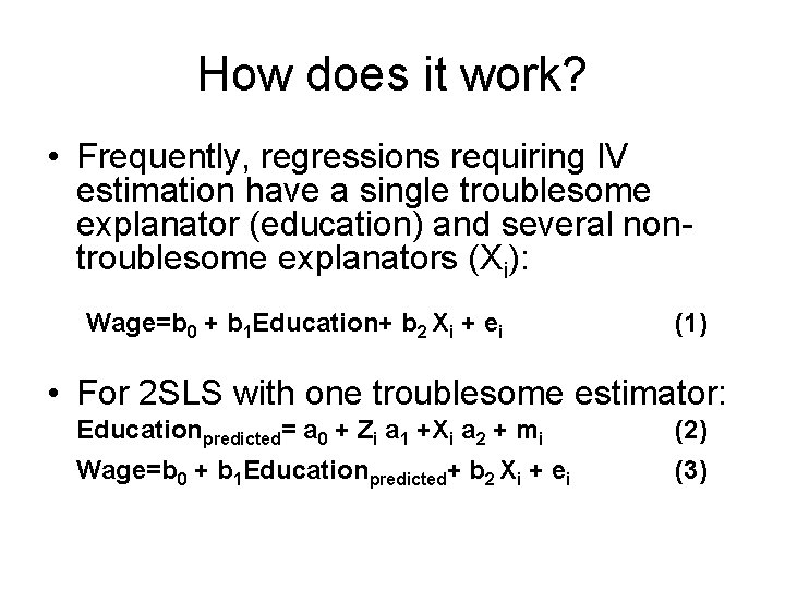
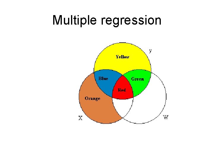
How does it work? • Frequently, regressions requiring IV estimation have a single troublesome explanator (education) and several nontroublesome explanators (Xi): Wage=b 0 + b 1 Education+ b 2 Xi + ei (1) • For 2 SLS with one troublesome estimator: Educationpredicted= a 0 + Zi a 1 +Xi a 2 + mi (2) Wage=b 0 + b 1 Educationpredicted+ b 2 Xi + ei (3)

Hence • To use the IV approach we need at least one additional variable, referred to as an instrument. The instrument has to satisfy two conditions: • i) Relevance (easy to test) • ii) Validity (cannot be tested)

Proposed instruments for education • Distance to college. • Quarter of birth with compulsory schooling.

Bad instruments • When the instruments are not valid. • Remember that this cannot be tested. • Overidentification tests are always used when possible but they can only help prove that an instrument is bad.

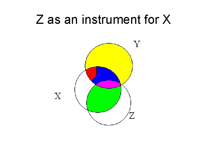
Weak instruments • We call an instrument weak if the correlation with the troublesome variable is low. • The main problem is that the variance of 2 SLS becomes greatly inflated.

Venn diagrams

Multiple regression

Z as an instrument for X

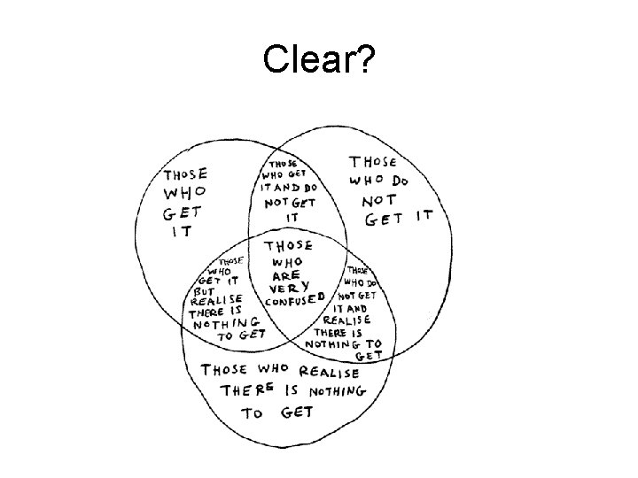
Clear?

Ugly instruments • What are we really measuring? • If heterogeneity is present, IV estimation may reveal results for a specific group which may differ from the average effect. • LATE: Local Average Treatment Effect.

Example • Effect of education. Those affected by school laws have a high marginal utility of an extra year. Thereby we are not measuring the returns to education in general. Not even the effect of education for those with low education. The effect is rather one for those who would not have studied the extra year absent the schooling law. • So, we must know what we are measuring!

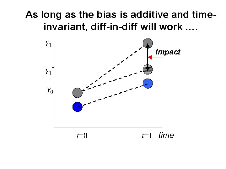
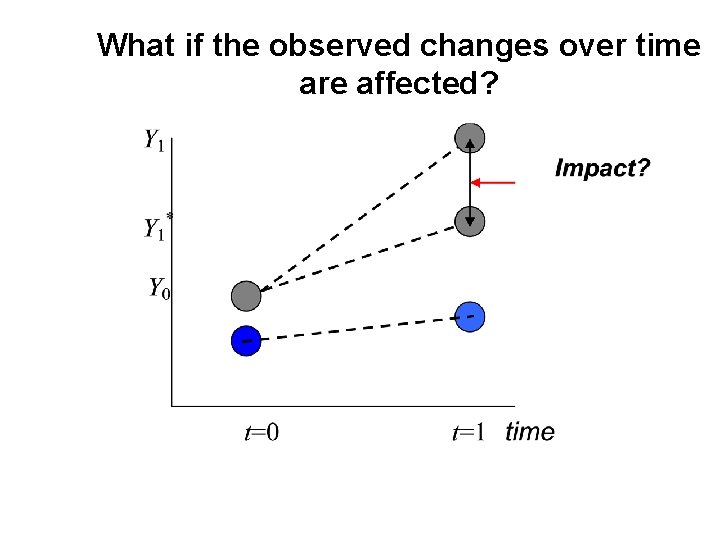
Difference in differences (DD) • Requires that data is available both before and after treatment. • Basic idea: Control for pre-period differences in outcomes between T and C. • Crucial assumption. Absent the treatment, the outcomes would have followed the same trend. • Main practical issue: Omitted variable… you must argue your case strongly!

As long as the bias is additive and timeinvariant, diff-in-diff will work ….

What if the observed changes over time are affected?

Problems • The main problem is that something else may have happened at the same time. • Or that the trends are different. • More periods is better.

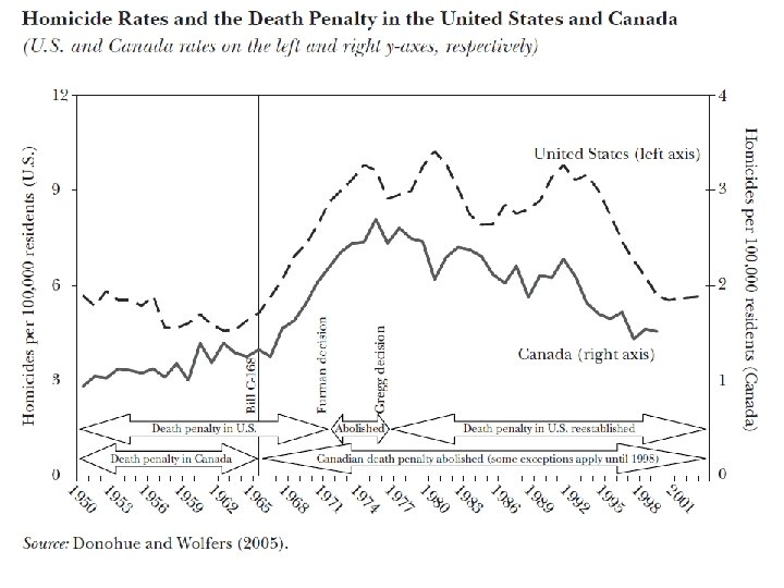
Real world example • Effect of the death penalty on homicide rates. • Donohue and Wolfers (2005) “Uses and abuses of empirical evidence in the death penalty debate”. • Use the trend in Canada as a counterfactual for the trend in the US

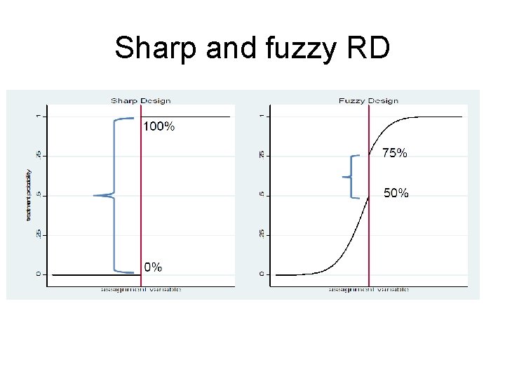
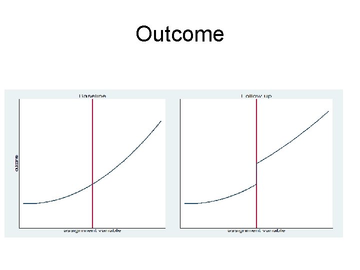
Regression Discontinuity (RD) • Basic idea: Exploit that the probability of treatment is a discontinuous function of at least one observable variable. • Clear right • The idea is to estimate the treatment effect using individuals just below the threshold as a control for those just above. • Examples may be that a poverty relief program is only given to those with less than 40 dollars per month or be that you get into a good university if your exam score is at least 207.

Sharp and fuzzy RD

Outcome

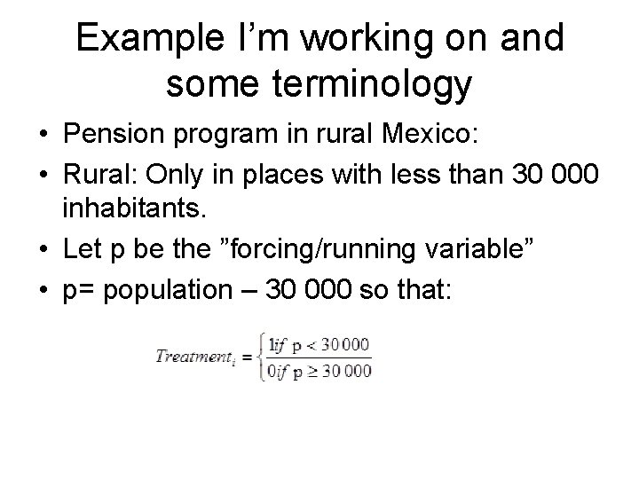
Example I’m working on and some terminology • Pension program in rural Mexico: • Rural: Only in places with less than 30 000 inhabitants. • Let p be the ”forcing/running variable” • p= population – 30 000 so that:

So, how do we estimate this? • Say we want to estimate the effects on poverty. • Example on the blackboard.

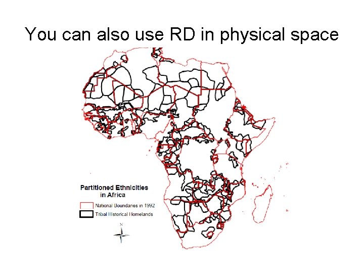
You can also use RD in physical space

RD • Very popular. • Often a much closer cousin of randomization than the other methods. • Also ethical advantage if distribution is based on needs. • Crucial assumption: No manipulation or sorting around the threshold.

RD • Underexploited: Cf. Burgess and Pande: • “Banks were required to select unbanked locations for branch expansion from a list circulated by the Central Bank. This list identified all unbanked locations with a population above a certain number. As the same population cut-off was applied across India. . . The list was updated, with a lower population cutoff, every three years. ” • They could have used RD.

Summary • Randomization requires minimal assumptions. • Non-experimental methods require assumptions that must be carefully assessed. • These assumptions cannot be proven so they must be very well argued. 70

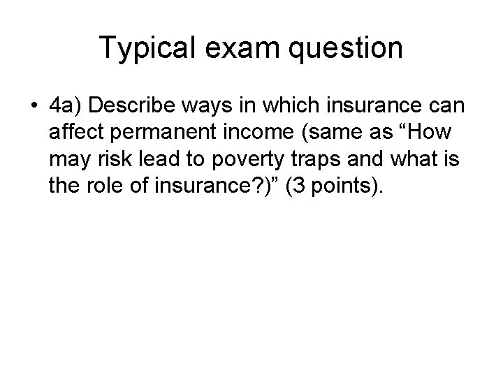
Typical exam question • 4 a) Describe ways in which insurance can affect permanent income (same as “How may risk lead to poverty traps and what is the role of insurance? )” (3 points).

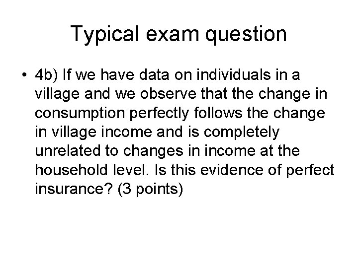
Typical exam question • 4 b) If we have data on individuals in a village and we observe that the change in consumption perfectly follows the change in village income and is completely unrelated to changes in income at the household level. Is this evidence of perfect insurance? (3 points)