Developing optimal diffuse pollution management strategies in an

Developing optimal diffuse pollution management strategies in an agricultural watershed under future climate change Dong Jin Jeon, Seo Jin Ki, Kyung Hwa Cho*, Joon Ha Kim† Environmental Systems Engineering Laboratory (ESEL) School of Environmental Science and Engineering, Gwangju Institute of Science and Technology (GIST) *School of Urban and Environmental Engineering, Ulsan National Institute of Science and Technology (UNIST)

Outline 1 Introduction 2 Methodology 3 Results 4 Conclusions 2

Introduction 3

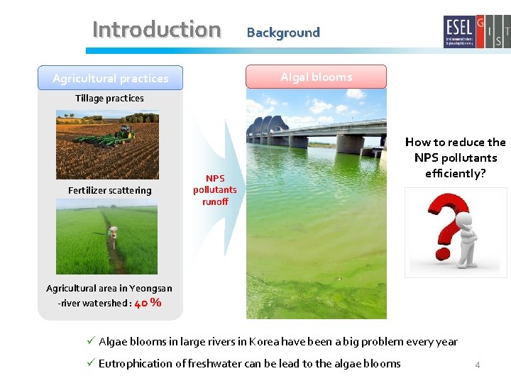
Introduction Background Algal blooms Agricultural practices Tillage practices Fertilizer scattering NPS pollutants runoff How to reduce the NPS pollutants efficiently? Agricultural area in Yeongsan -river watershed : 40 % ü Algae blooms in large rivers in Korea have been a big problem every year ü Eutrophication of freshwater can be lead to the algae blooms 4

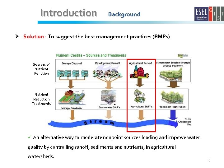
Introduction Background Ø Solution : To suggest the best management practices (BMPs) Sources of Nutrient Pollution Nutrient Reduction Treatments ü An alternative way to moderate nonpoint sources loading and improve water quality by controlling runoff, sediments and nutrients, in agricultural watersheds. 5

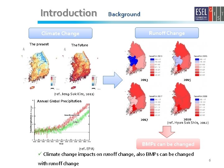
Introduction Background Runoff Change Climate Change The present The future 2013 2015 2017 2020 (ref. Hyun Suk Shin, 2012) (ref. Jong-Suk Kim, 2011) Annual Global Precipitation (ref. EPA) BMPs can be changed ü Climate change impacts on runoff change, also BMPs can be changed with runoff change 6

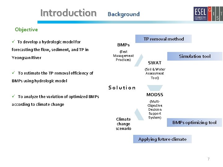
Introduction Background Objective ü To develop a hydrologic model forecasting the flow, sediment, and TP in Yeongsan River BMPs (Best Management Practices) TP removal method Simulation tool SWAT (Soil & Water Assessment Tool) ü To estimate the TP removal efficiency of BMPs using hydrologic model Solution MODSS ü To analyze the variation of optimized BMPs according to climate change Climate change scenario (Multi. Objective Decision Support System) BMPs optimizing tool Applying future climate 7

Methodology 8

Methodology Site Description § Area [km 2] : 724. 37 § The number of sub-basins : 9 § The number of agricultural HRU : 98 § The number of Rice HRU : 39 § The number of Soybean HRU : 59 Land Use 0 5 km Area (%) Forest-Evergreen 24. 85 Rice 21. 08 Forest-Mixed 12. 34 Forest-Deciduous 10. 94 Soybean 8. 66 Residential-High Density 7. 87 ü HRU(Hydrologic Response Unit) is classified by land use, slope, and soil component 9

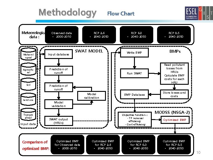
Methodology Flow Chart Meteorological data : Meteorol ogical Input database Agricultu ral Prediction of runoff Soil Prediction of runoff Input data SWAT MODEL Model calibration Land use Topogra phical RCP 2. 6 • 2040 -2050 Observed data • 2000 -2010 RCP 6. 0 • 2040 -2050 Write BMP RCP 8. 5 • 2040 -2050 BMPs Run SWAT Read pollutant losses from HRUs Calculate BMP costs for each HRU BMP Database Store losses and costs Model validation Objective function : - TP removal efficiency - Cost efficiency SWAT output (HRUs) Comparison of optimized BMP: Optimized BMP for Observed data • 2000 -2010 Optimized BMP for RCP 2. 6 • 2040 -2050 Optimized BMP for RCP 6. 0 • 2040 -2050 MODSS (NSGA-2) Optimized BMP for RCP 8. 5 • 2040 -2050 10

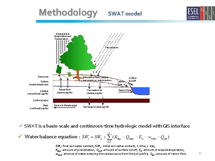
Methodology SWAT model Evaporation and Transpiration Precipitation Root zone Infiltration/Plant uptake/ Soil moisture redistribution Vadose (unsaturated) zone Shallow (unconfined) aquifer Revap from shallow aquifer Percolation to shallow aquifer Lateral Flow Surface Runoff Return Flow Confining layer Deep (confined) aquifer Flow out of watershed Recharge to deep aquifer ü SWAT is a basin-scale and continuous-time hydrologic model with GIS interface ü Water balance equation : SWt: final soil water content, SWo: initial soil water content, t: time, i: day, Rday: amount of precipitation, Qsurf: amount of surface runoff, Ea: amount of evapotranspiration, wseep: amonut of water entering the vadose zone from the soil profile, Qgw: amount of return flow 11

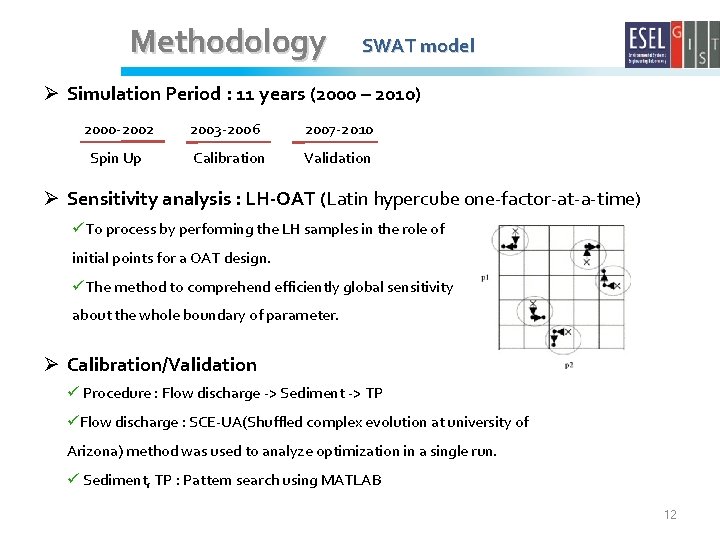
Methodology SWAT model Ø Simulation Period : 11 years (2000 – 2010) 2000 -2002 2003 -2006 2007 -2010 Spin Up Calibration Validation Ø Sensitivity analysis : LH-OAT (Latin hypercube one-factor-at-a-time) üTo process by performing the LH samples in the role of initial points for a OAT design. üThe method to comprehend efficiently global sensitivity about the whole boundary of parameter. Ø Calibration/Validation ü Procedure : Flow discharge -> Sediment -> TP üFlow discharge : SCE-UA(Shuffled complex evolution at university of Arizona) method was used to analyze optimization in a single run. ü Sediment, TP : Pattern search using MATLAB 12

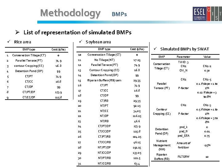
Methodology BMPs Ø List of representation of simulated BMPs ü Rice area ü Soybean area BMP type Cost ($/ha) 10 Conservation Tillage (CT) 0 74. 9 11 No Tillage (NT) 17. 25 contour Cropping (CC) 16. 8 12 Parallel Terrace (PT) 74. 9 4 Detention Pond (DP) 99 13 Contour Cropping (CC) 16. 8 5 CT/PT 74. 9 14 Detention Pond (DP) 99 6 CT/CC 16. 8 15 Riparian Buffers (RB) 10 m 29. 35 7 CT/DP 99 16 CT/PT 74. 9 8 CT/PT/DP 173. 9 17 CT/CC 16. 8 9 CT/CC/DP 115. 8 18 CT/DP 99 19 CT/RB 29. 35 20 NT/PT 92. 15 21 NT/CC 34. 05 22 NT/DP 116. 25 23 NT/RB 46. 6 24 CT/PT/DP 173. 9 25 CT/CC/DP 115. 8 26 CT/PT/RB 104. 25 27 CT/CC/RB 46. 15 28 NT/PT/DP 191. 15 29 NT/CC/DP 133. 05 30 NT/PT/RB 121. 5 31 NT/CC/RB 63. 4 BMP type Cost ($/ha) 1 Conservation Tillage (CT) 0 2 Parallel Terrace (PT) 3 ü Simulated BMPs by SWAT BMP Parameter Value Conservation Tillage (CT) Till ID: 3 CN 2 OV_N CN 2 -2 0. 30 CN 2 -5 0. 1 if slope = 1 to 2% 0. 12 if slope = 3 to 8% Parallel Terrace (PT) P-factor CN 2 -3 0. 5 if slope = 1 to 2% 0. 6 if slope = 3 to 8% Detention Pond (DP) pnd_k pnd_fr pnd_ESA 0 0. 01 0. 75 Nutrient Management (NM) Amount of fertilizer -25% Riparian Buffers (RB) FILTERW 10 Contour Cropping (CC)

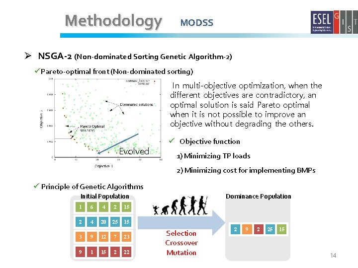
Methodology MODSS Ø NSGA-2 (Non-dominated Sorting Genetic Algorithm-2) üPareto-optimal front (Non-dominated sorting) In multi-objective optimization, when the different objectives are contradictory, an optimal solution is said Pareto optimal when it is not possible to improve an objective without degrading the others. Evolved ü Objective function 1) Minimizing TP loads 2) Minimizing cost for implementing BMPs ü Principle of Genetic Algorithms Initial Population 1 6 4 2 15 2 4 20 25 15 3 9 12 7 23 9 1 15 2 22 Dominance Population Selection Crossover Mutation 2 9 2 25 15 14

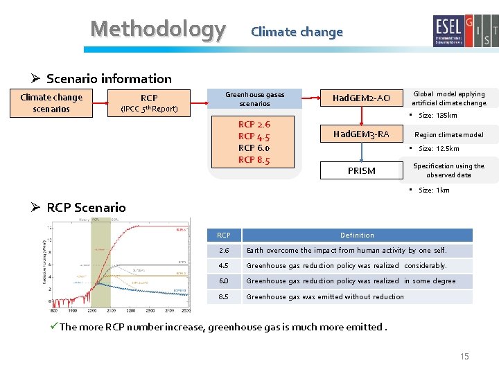
Methodology Climate change Ø Scenario information Climate change scenarios RCP (IPCC 5 th Report) Greenhouse gases scenarios RCP 2. 6 RCP 4. 5 RCP 6. 0 RCP 8. 5 Had. GEM 2 -AO Global model applying artificial climate change • Size: 135 km Had. GEM 3 -RA Region climate model • Size: 12. 5 km PRISM Specification using the observed data • Size: 1 km Ø RCP Scenario RCP Definition 2. 6 Earth overcome the impact from human activity by one self. 4. 5 Greenhouse gas reduction policy was realized considerably. 6. 0 Greenhouse gas reduction policy was realized in some degree 8. 5 Greenhouse gas was emitted without reduction üThe more RCP number increase, greenhouse gas is much more emitted. 15

Results 16

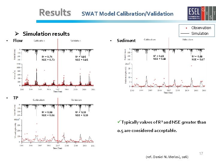
Results SWAT Model Calibration/Validation Ø Simulation results • • . Observation Simulation Flow • R 2 = 0. 74 NSE = 0. 73 R 2 = 0. 85 NSE = 0. 85 R 2 = 0. 58 NSE = 0. 56 R 2 = 0. 39 NSE = 0. 39 Sediment R 2 = 0. 69 NSE = 0. 68 R 2 = 0. 68 NSE = 0. 67 TP üTypically values of R 2 and NSE greater than 0. 5 are considered acceptable. (ref. Daniel N. Moriasi, 206) 17

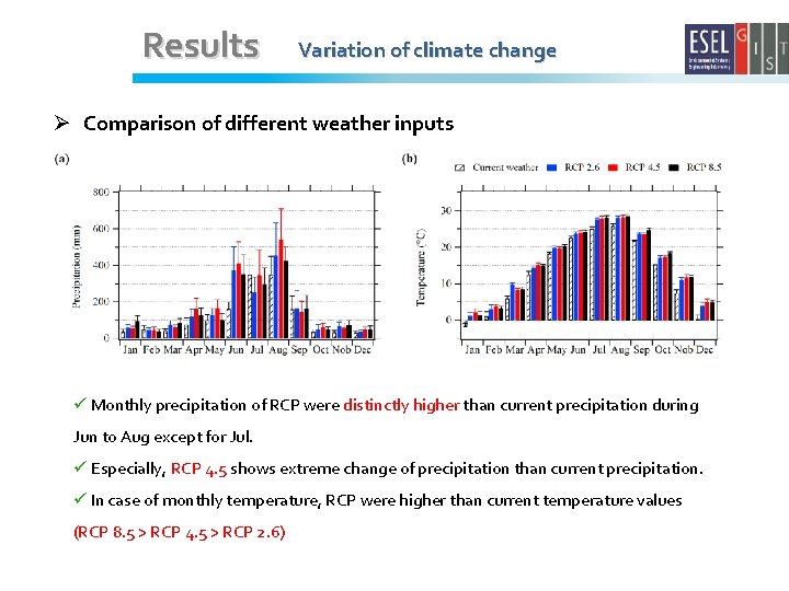
Results Variation of climate change Ø Comparison of different weather inputs ü Monthly precipitation of RCP were distinctly higher than current precipitation during Jun to Aug except for Jul. ü Especially, RCP 4. 5 shows extreme change of precipitation than current precipitation. ü In case of monthly temperature, RCP were higher than current temperature values (RCP 8. 5 > RCP 4. 5 > RCP 2. 6)

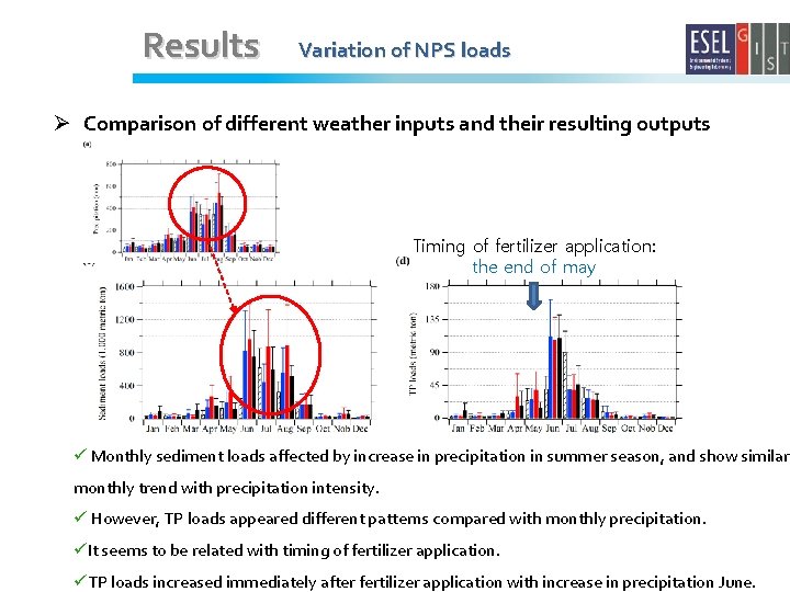
Results Variation of NPS loads Ø Comparison of different weather inputs and their resulting outputs Timing of fertilizer application: the end of may ü Monthly sediment loads affected by increase in precipitation in summer season, and show similar monthly trend with precipitation intensity. ü However, TP loads appeared different patterns compared with monthly precipitation. üIt seems to be related with timing of fertilizer application. üTP loads increased immediately after fertilizer application with increase in precipitation June.

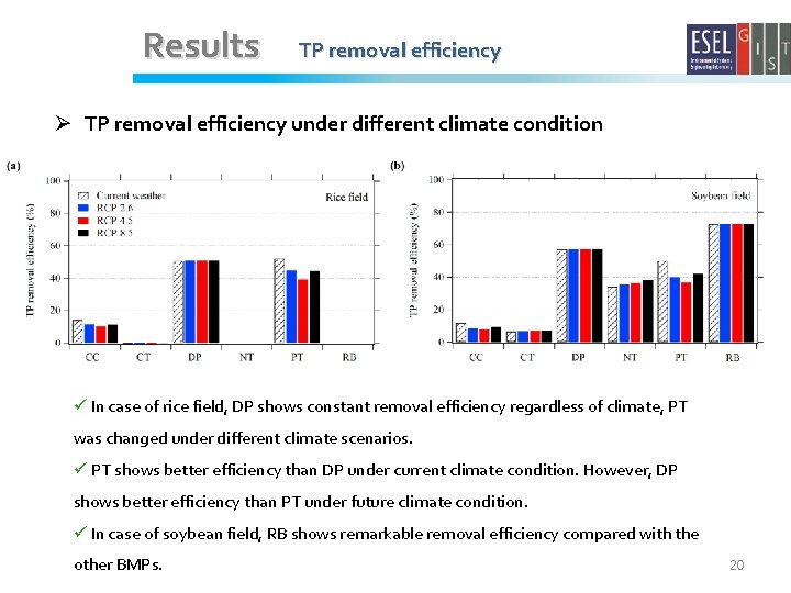
Results TP removal efficiency Ø TP removal efficiency under different climate condition ü In case of rice field, DP shows constant removal efficiency regardless of climate, PT was changed under different climate scenarios. ü PT shows better efficiency than DP under current climate condition. However, DP shows better efficiency than PT under future climate condition. ü In case of soybean field, RB shows remarkable removal efficiency compared with the other BMPs. 20

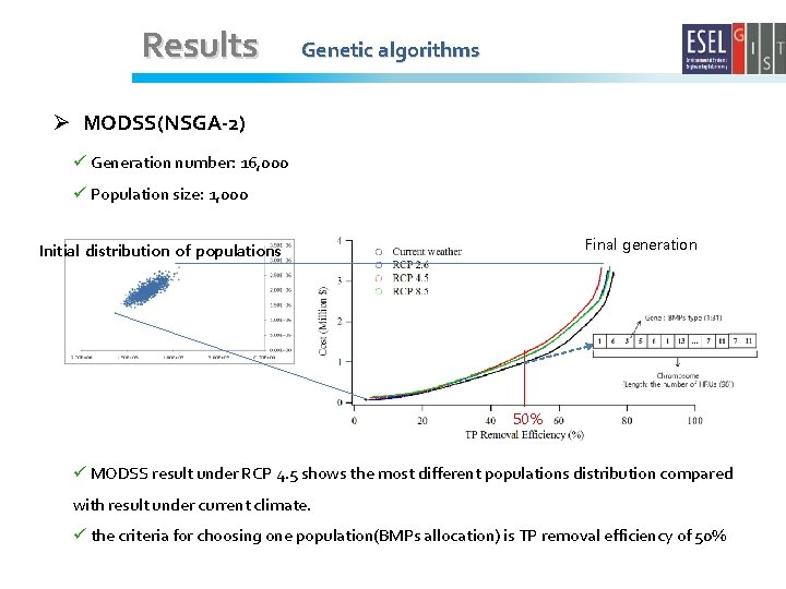
Results Genetic algorithms Ø MODSS(NSGA-2) ü Generation number: 16, 000 ü Population size: 1, 000 Final generation Initial distribution of populations 50% ü MODSS result under RCP 4. 5 shows the most different populations distribution compared with result under current climate. ü the criteria for choosing one population(BMPs allocation) is TP removal efficiency of 50%

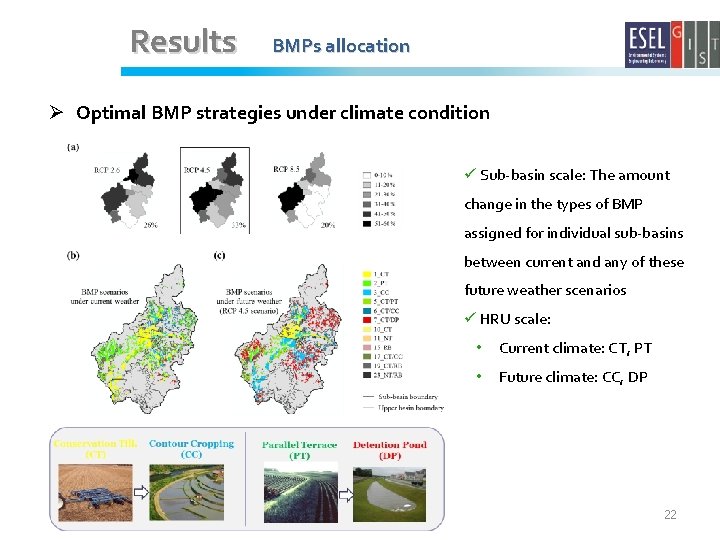
Results BMPs allocation Ø Optimal BMP strategies under climate condition ü Sub-basin scale: The amount change in the types of BMP assigned for individual sub-basins between current and any of these future weather scenarios ü HRU scale: • Current climate: CT, PT • Future climate: CC, DP 22

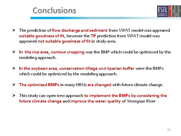
Conclusions Ø The prediction of flow discharge and sediment from SWAT model was appeared suitable goodness of fit, however the TP prediction from SWAT model was appeared not suitable goodness of fit in study area. Ø In the rice area, contour cropping was the BMP which could be optimized by the modeling approach. Ø In the soybean area, conservation tillage and riparian buffer were the BMPs which could be optimized by the modeling approach. Ø The optimized BMPs in many HRUs are changed with future climate change. Ø This study can open new approach to implement the BMPs by considering the future climate change and improve the water quality of Yeongsan River 23

Thank you 24

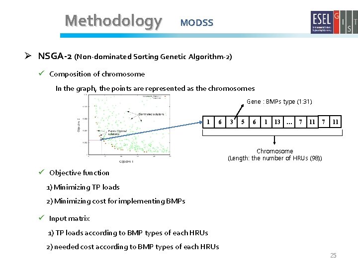
Methodology MODSS Ø NSGA-2 (Non-dominated Sorting Genetic Algorithm-2) ü Composition of chromosome In the graph, the points are represented as the chromosomes Gene : BMPs type (1: 31) 1 6 3 5 6 1 13 … 7 11 Chromosome (Length: the number of HRUs (98)) ü Objective function 1) Minimizing TP loads 2) Minimizing cost for implementing BMPs ü Input matrix 1) TP loads according to BMP types of each HRUs 2) needed cost according to BMP types of each HRUs 25

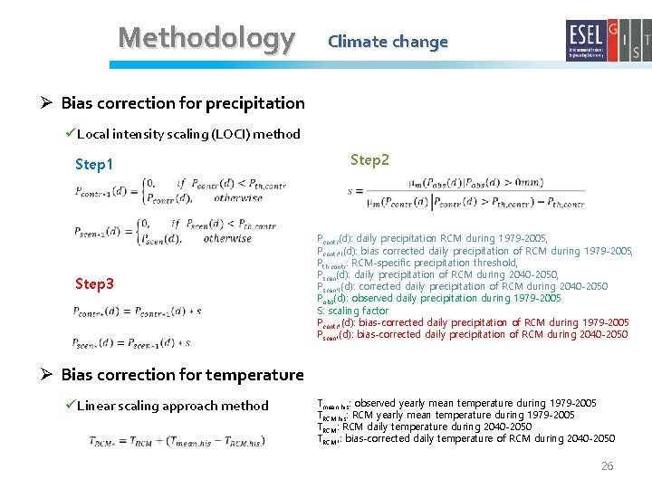
Methodology Climate change Ø Bias correction for precipitation üLocal intensity scaling (LOCI) method Step 2 Step 1 Step 3 Pcontr(d): daily precipitation RCM during 1979 -2005, Pcontr*I(d): bias corrected daily precipitation of RCM during 1979 -2005, Pth. contr: RCM-specific precipitation threshold, Pscen(d): daily precipitation of RCM during 2040 -2050, Pscen*I(d): corrected daily precipitation of RCM during 2040 -2050 Pobs(d): observed daily precipitation during 1979 -2005 S: scaling factor Pcontr*(d): bias-corrected daily precipitation of RCM during 1979 -2005 Pscen*(d): bias-corrected daily precipitation of RCM during 2040 -2050 Ø Bias correction for temperature üLinear scaling approach method Tmean. his: observed yearly mean temperature during 1979 -2005 TRCM. his: RCM yearly mean temperature during 1979 -2005 TRCM: RCM daily temperature during 2040 -2050 TRCM*: bias-corrected daily temperature of RCM during 2040 -2050 26

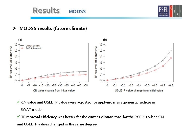
Results MODSS Ø MODSS results (future climate) ü CN value and USLE_P value were adjusted for applying management practices in SWAT model. ü TP removal efficiency was better for the current climate than for the RCP 4. 5 when CN and USLE_P values changed in the same degree.