Developing a DSP Core using an FPGA Prototype

Developing a DSP Core using an FPGA Prototype for Scintillation Detector Signals Prepared by: Eng. Mahmoud Kamel Submitted to: Communication & Electronics Dept. , Al Azhar University Supervised by: Prof. Dr. Ahmed Safwat Prof. Dr. Mahmoud Ashour Dr. Ashraf Aboshosha

Outline • This core gives us all important features of the scintillation detector signals such as shaping, counting, pulse height and multichannel analyzing. • The main purpose of this research work is to de-noise, compress and reconstruct the scintillation signals by which the processing speed, storage and precision will be improved. 3

Outline • This core is implemented to apply the forward wavelet transform and interpolation technique. A new contribution of this framework arises from employing the interpolation techniques to reconstruct the signals where the mother wavelet and details are not required. • Building a Multi-Channel Analyzer of the scintillation detector signals 4

Index of Content • • Scintillation detectors Importance of scintillation detectors Data Acquisition System Proposed digital processing algorithm Wavelets – Interpolation Technique Comparative study with the previous techniques Single channel and multi channel analyzer Conclusions and future work 5

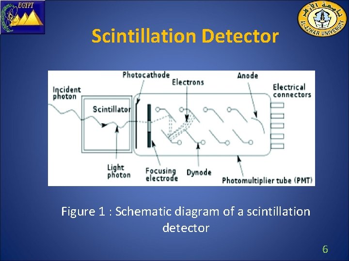
Scintillation Detector Figure 1 : Schematic diagram of a scintillation detector 6

Scintillation Detector • A scintillator is a material that emits light, scintillates, when absorbing radiation. • The energy can be determined by measuring the pulse height spectrum. This is called spectroscopy. • A scintillation detector is obtained when a scintillator is coupled to an electronic light sensor such as PMT or photodiode. 7

Importance of Scintillation Detectors • Detection of mixed ionizing fluxes near nuclear objects. • Radionuclide control of samples and radiation pollution. • Determination of the type and energy of high -energy particles and products of their reactions with targets. • Nuclear medicine (Gamma Camera, PET Tomography, …) 8

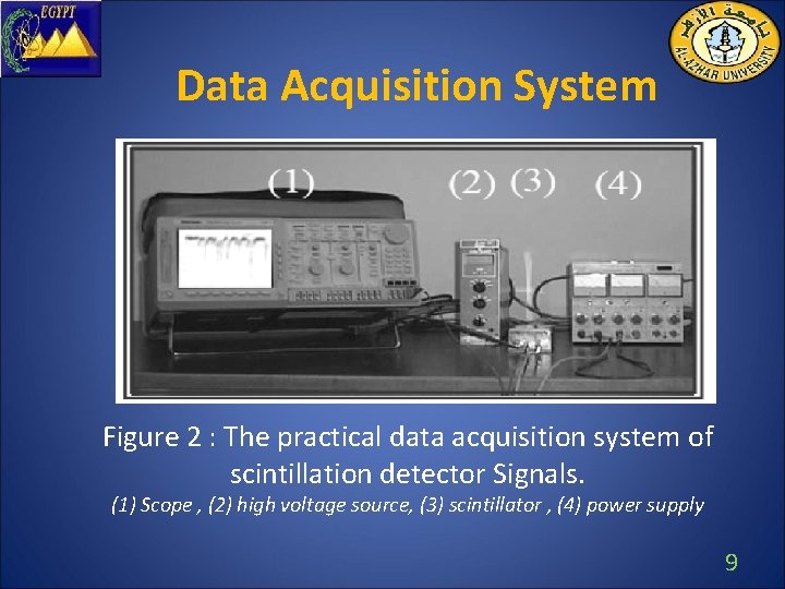
Data Acquisition System Figure 2 : The practical data acquisition system of scintillation detector Signals. (1) Scope , (2) high voltage source, (3) scintillator , (4) power supply 9

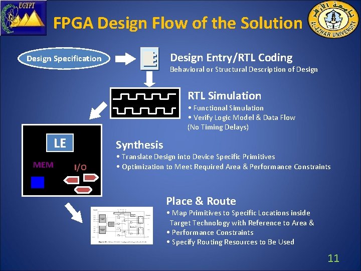
Why FPGA ? • FPGA incorporates thousands of logic cells linked by programmable switches • Highly parallel configurable digital signal processor • A many channel signal processing was required in these detector to obtain a precise signals • Availability of high-level design entry method • FPGA designs easily changed, recompiled and low cost 10

FPGA Design Flow of the Solution Design Entry/RTL Coding Design Specification Behavioral or Structural Description of Design RTL Simulation • Functional Simulation • Verify Logic Model & Data Flow (No Timing Delays) LE MEM Synthesis I/O • Translate Design into Device Specific Primitives • Optimization to Meet Required Area & Performance Constraints Place & Route • Map Primitives to Specific Locations inside Target Technology with Reference to Area & • Performance Constraints • Specify Routing Resources to Be Used 11

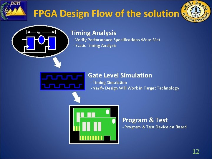
FPGA Design Flow of the solution tclk Timing Analysis - Verify Performance Specifications Were Met - Static Timing Analysis Gate Level Simulation - Timing Simulation - Verify Design Will Work in Target Technology Program & Test - Program & Test Device on Board 12

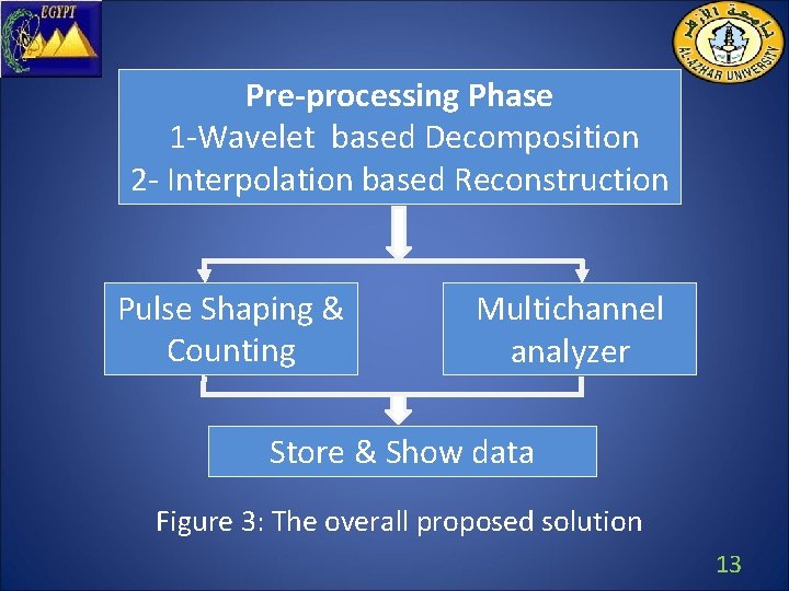
Pre-processing Phase 1 -Wavelet based Decomposition 2 - Interpolation based Reconstruction Pulse Shaping & Counting Multichannel analyzer Store & Show data Figure 3: The overall proposed solution 13

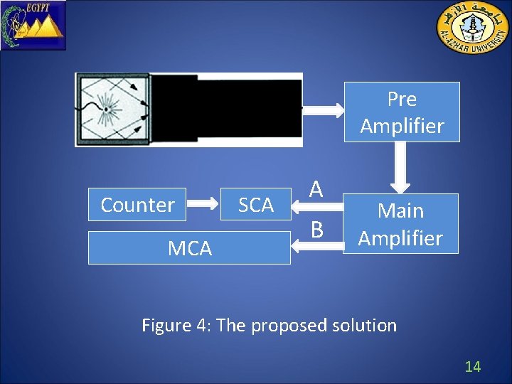
Pre Amplifier Counter MCA SCA A B Main Amplifier Figure 4: The proposed solution 14

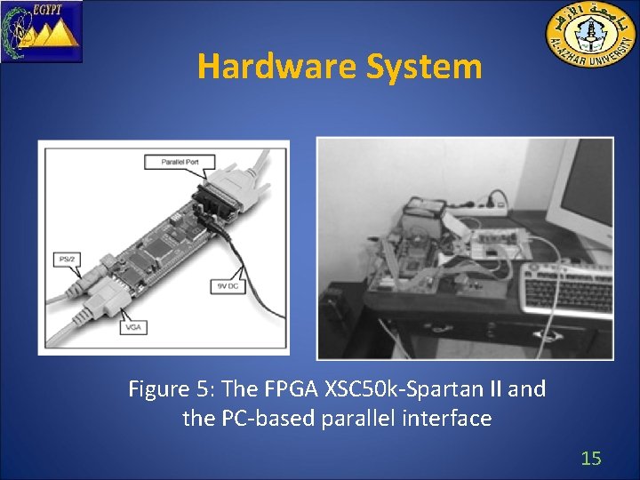
Hardware System Figure 5: The FPGA XSC 50 k-Spartan II and the PC-based parallel interface 15

Pre-processing Phase • De-noising • Compression • Reconstruction 16

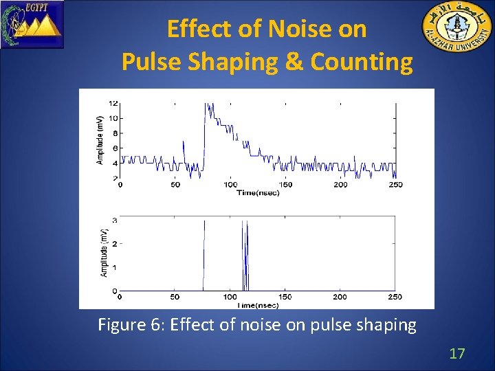
Effect of Noise on Pulse Shaping & Counting Figure 6: Effect of noise on pulse shaping 17

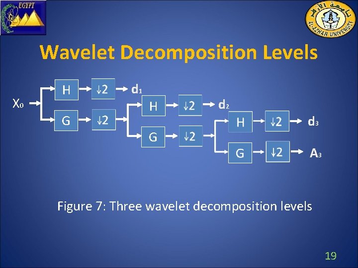
Wavelets • The wavelet analysis procedure is to adopt a wavelet prototype function, called an analyzing wavelet or mother wavelet. • Wavelet transform decompose the original signal into different scales of resolution; these called the approximation and detail coefficients. 18

Wavelet Decomposition Levels X 0 H G d 1 H G d 2 d 3 A 3 Figure 7: Three wavelet decomposition levels 19

Wavelet Families • • • Haar Daubechies Biorthogonal Coifelt Symelet Myer 20

Haar Wavelet Design Pro: • Allows good approximation with a subset of coefficients. • It can be computed quickly and easily. • Implemented easily by FPGA. 21

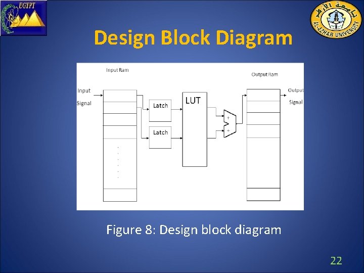
Design Block Diagram Figure 8: Design block diagram 22

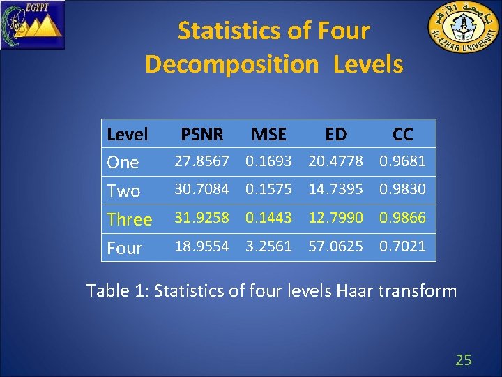
Selecting the best Decomposition Level • The quality of the compressed signals is the main criterion to select the best decomposition level in terms of Peak Signal to Noise Ratio (PSNR). • The other similarity measure are Euclidean Distance (ED) , Cross Correlation coefficient (CC) and Mean Square Error(MSE). 23

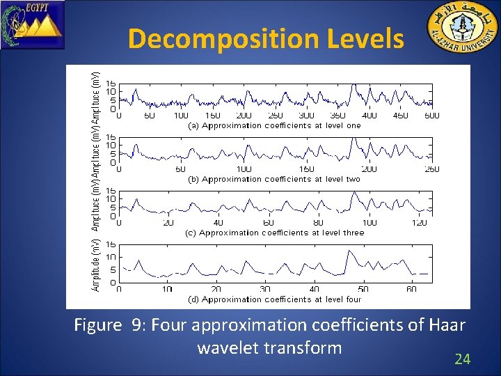
Decomposition Levels Figure 9: Four approximation coefficients of Haar wavelet transform 24

Statistics of Four Decomposition Levels Level One Two Three Four PSNR MSE ED CC 27. 8567 0. 1693 20. 4778 0. 9681 30. 7084 0. 1575 14. 7395 0. 9830 31. 9258 0. 1443 12. 7990 0. 9866 18. 9554 3. 2561 57. 0625 0. 7021 Table 1: Statistics of four levels Haar transform 25

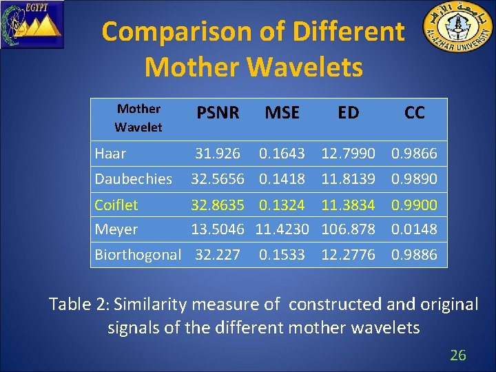
Comparison of Different Mother Wavelets Mother Wavelet PSNR MSE ED CC Haar 31. 926 Daubechies 32. 5656 0. 1418 11. 8139 0. 9890 Coiflet Meyer 32. 8635 0. 1324 11. 3834 0. 9900 13. 5046 11. 4230 106. 878 0. 0148 Biorthogonal 32. 227 0. 1643 12. 7990 0. 9866 0. 1533 12. 2776 0. 9886 Table 2: Similarity measure of constructed and original signals of the different mother wavelets 26

Interpolation • The Interpolation is a method of constructing new data points within the range of a discrete set of known data points. • Interpolation is performed by fitting the supplied data with polynomial functions between data points and evaluating the appropriate function at the desired points. 27

Reconstruct Signals Using Interpolation Figure 10: a) Original signals. b) Transformed signal. c) Reconstructed signals 28

Interpolation Algorithms • • Nearest neighbor interpolation Linear interpolation Cubic Hermit Interpolation Cubic spline interpolation 29

Comparison of Applying Different Interpolation Techniques PSNR MSE ED CC 29. 7192 0. 2731 16. 4669 0. 9782 Cubic Spline 31. 9258 27. 8501 Nearst Cubic Hermit 30. 6066 0. 1643 12. 7990 0. 9866 0. 8380 28. 8462 0. 9307 0. 2226 14. 8984 0. 9818 Method Linear Table 3: Statistics of different interpolation techniques 30

Previous Pre-processing Techniques 1. Accumulation Technique 2. Median filter 31

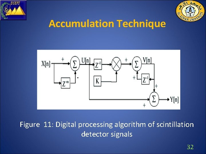
Accumulation Technique Figure 11: Digital processing algorithm of scintillation detector signals 32

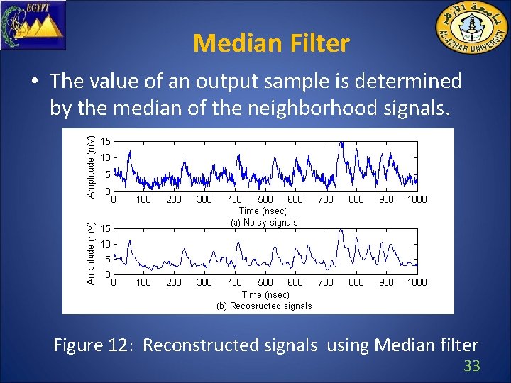
Median Filter • The value of an output sample is determined by the median of the neighborhood signals. Figure 12: Reconstructed signals using Median filter 33

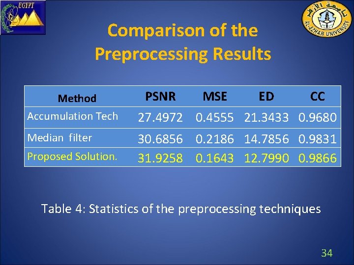
Comparison of the Preprocessing Results Method Accumulation Tech Median filter Proposed Solution. PSNR MSE ED CC 27. 4972 0. 4555 21. 3433 0. 9680 30. 6856 0. 2186 14. 7856 0. 9831 31. 9258 0. 1643 12. 7990 0. 9866 Table 4: Statistics of the preprocessing techniques 34

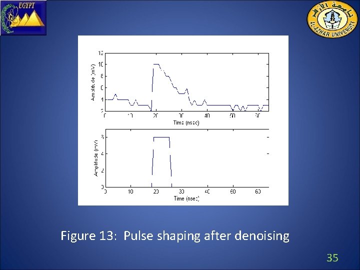
Figure 13: Pulse shaping after denoising 35

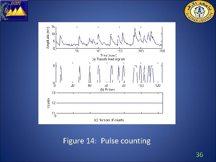
Figure 14: Pulse counting 36

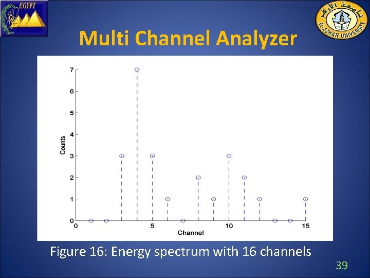
Multi Channel Analyzer • The MCA system is used to measure the height of each output pulse and the number of each output pulses simultaneously. • By performing this operation for all detector events in a given interval the MCA generates a spectrum of the distribution of energy for a measured events with the y axis representing counts and the x axis representing channel value. 37

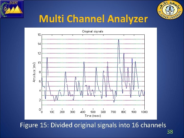
Multi Channel Analyzer Figure 15: Divided original signals into 16 channels 38

Multi Channel Analyzer Figure 16: Energy spectrum with 16 channels 39

Channel Calibration • Energy channel values are converted into kilo electron volts with a channel-to-kilo electron volt conversion factor which is determined from a comparison of photo peak energies and channel location close to the energy of interest. 40

Conclusions • One of the most important advantages of this system is the high compression rate (12. 5%) using the interpolated wavelets • Compared with the accumulation technique and median filtering, the proposed design achieved the best precision • Capability of constructing MCA from SCA • Coiflet is the best mother wavelet and Cubic spline is the best interpolation technique. Combining both of them for down and up sapling in wavelets is a new theoretical contribution of this framework 41

Future work • Applying more complex wavelet filters. • Modifying the proposed architecture to process more scintillator detectors. • Employing the presented results as a base to identify radiation type and isotopes. 42

Thank You