Determination Of Equilibrium Level Of Income Y Or

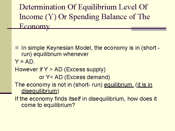
Determination Of Equilibrium Level Of Income (Y) Or Spending Balance of The Economy n In simple Keynesian Model, the economy is in (short - run) equilibrium whenever Y = AD. However if Y > AD (Excess supply) or Y< AD (Excess demand) The economy is not in (short- run) equilibrium. (it is in disequilibrium) If the economy finds itself in disequilibrium, how does it come to equilibrium?

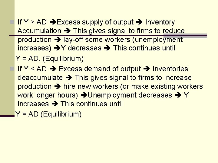
n If Y > AD Excess supply of output Inventory Accumulation This gives signal to firms to reduce production lay-off some workers (unemployment increases) Y decreases This continues until Y = AD. (Equilibrium) n If Y < AD Excess demand of output Inventories deaccumulate This gives signal to firms to increase production hire new workers (or make existing workers work longer hours) Unemployment decreases Y increases This continues until Y = AD (Equilibrium)

n Now we want to show this graphically and understand better the dynamics of adjustment to a new point of equilibrium from an old point of equilibrium:

The Case of Fiscal Policy n Suppose that we want to analyze the impact of Expansionary Fiscal Policy on the equilibrium values of Y, C, S, T, M, B. D (Budget deficit), I and X (Net Exports) of the economy: We will show it graphically and also understand the impact of such a policy intuitively based on theoretical relationships that we developed.

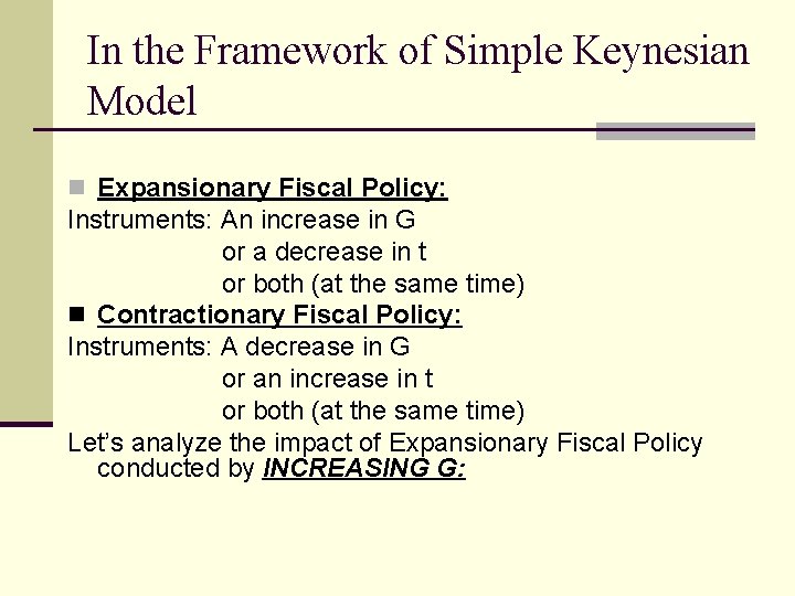
In the Framework of Simple Keynesian Model n Expansionary Fiscal Policy: Instruments: An increase in G or a decrease in t or both (at the same time) n Contractionary Fiscal Policy: Instruments: A decrease in G or an increase in t or both (at the same time) Let’s analyze the impact of Expansionary Fiscal Policy conducted by INCREASING G:

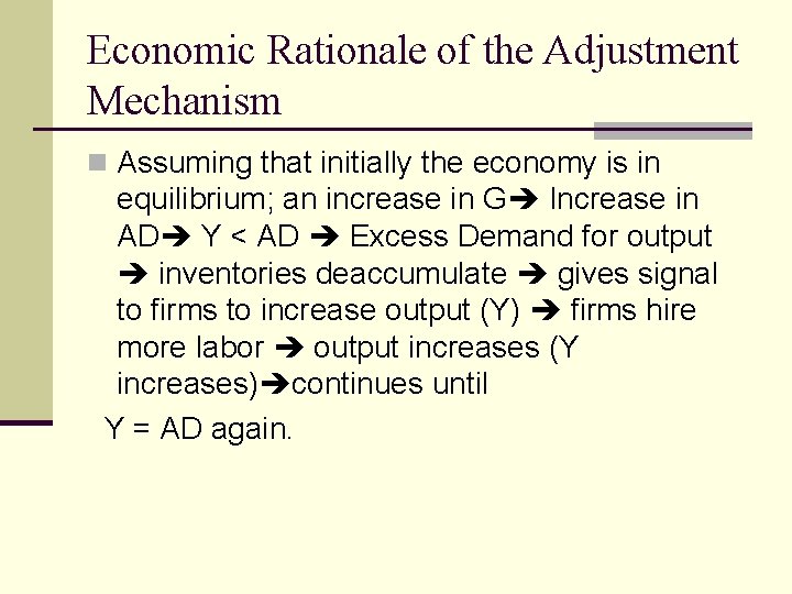
Economic Rationale of the Adjustment Mechanism n Assuming that initially the economy is in equilibrium; an increase in G Increase in AD Y < AD Excess Demand for output inventories deaccumulate gives signal to firms to increase output (Y) firms hire more labor output increases (Y increases) continues until Y = AD again.

Economic Rationale of the Adjustment Mechanism (Cont’d) n However as Y increases C, S, T and M all increase as well! n WHY? n Because C = f (Y), T = f (Y) S = f (Y), M = f (Y) in our Keynesian Model. What happens to Investment (I)? If I is autonomous of Y (as we assumed) there is no change in I.

n However since M increases as Y increases, X decreases because n X = g – m. Y where g=Exports n And M (imports)= m. Y!

How about BUDGET DEFICIT of the government? BD = G – T If G > T BD > 0 (Budget deficit) If G < T BD < 0 (Budget surplus) As G increases, initially BD increases ( or B. Surplus decreases) n But as Y increases this increases T leading to a decrease in BD. So the net effect of an increase in G and BD is ambiguous. n So what are the net effects of an increase in G? n n

Net effects of an increasing G n Equilibrium values of Y, C, S, M, T all increase relative to their levels at the initial equilibrium point. n Unemployment decreases, Net Exports (X) decrease, n (Trade balance deteriorates) n Net ∆ in BD is ambiguous n

n WE NOTE THAT: n Adjustment mechanism in response to other types of shocks such as changes in other autonomous components of AD is exactly same

HOME-WORK n Analyse the impact of each one of the following on equilibrium levels of Y, C, S, I, T, B. D, X, M and unemployment

HOME-WORK (Cont’d) An increase in Autonomous part of consumption expenditures b) An increase in foreign demand for exports c) A decrease in G d) An increase in Investment Spending due to more optimistic expectations about the future e) A decrease in t (income tax rate) Use graphs and explain the economic rationale of the adjustment mechanism and the net effects! a)

CASE 2: The impact of Contractionary Fiscal Policy (Case of increase in t) n Step by step explanation of adjustment mechanism n Higher t higher tax payments by households (T increases) A decrease in Disposable Income (Yd) lower C (and lower S) A decrease in AD Excess Supply of output (Y > AD) Inventory Accumulation gives signal to firms to decrease Y and lay-off workers Y decreases and unemployment increases As Y decreases, C, S, T, M decrease n This process continues until Y=AD n Converges to new equilibrium n Now we show this adjustment graphically on blackboard

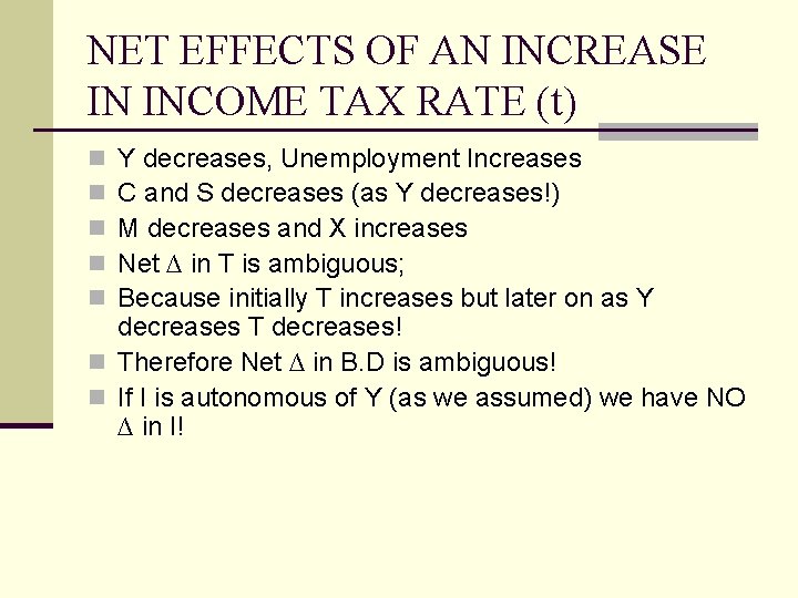
NET EFFECTS OF AN INCREASE IN INCOME TAX RATE (t) Y decreases, Unemployment Increases C and S decreases (as Y decreases!) M decreases and X increases Net ∆ in T is ambiguous; Because initially T increases but later on as Y decreases T decreases! n Therefore Net ∆ in B. D is ambiguous! n If I is autonomous of Y (as we assumed) we have NO ∆ in I! n n n