Detecting Gravitational Waves with a Pulsar Timing Array

Detecting Gravitational Waves with a Pulsar Timing Array LINDLEY LENTATI CAMBRIDGE UNIVERSITY

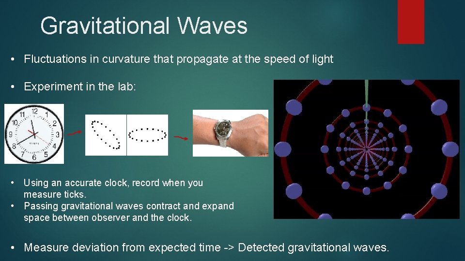
Gravitational Waves • Fluctuations in curvature that propagate at the speed of light • Experiment in the lab: • Using an accurate clock, record when you measure ticks. • Passing gravitational waves contract and expand space between observer and the clock. • Measure deviation from expected time -> Detected gravitational waves.

One problem. . • Expected length change: width of an atomic nucleus in one meter baseline • Need *very* accurate clock • Or huge distances… • Segue into….

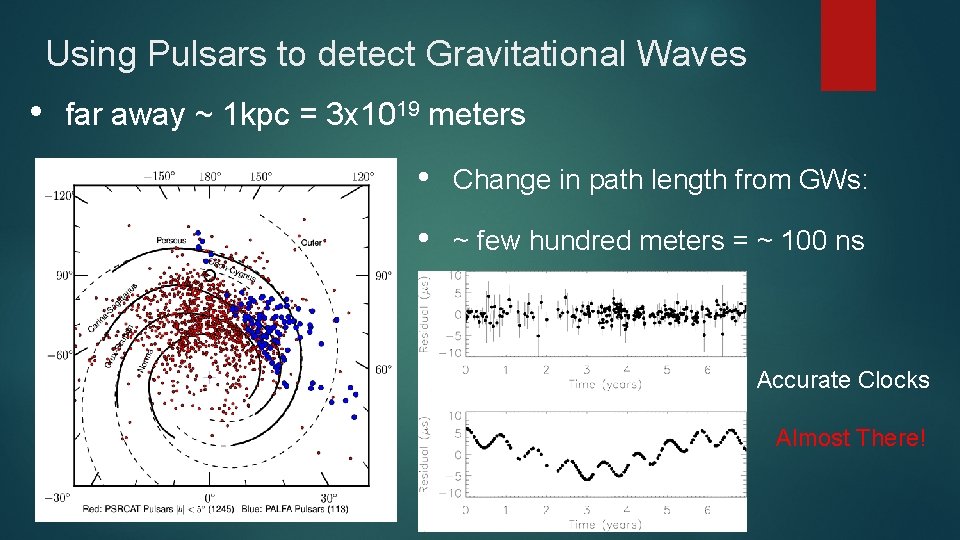
Using Pulsars to detect Gravitational Waves • far away ~ 1 kpc = 3 x 1019 meters • Change in path length from GWs: • ~ few hundred meters = ~ 100 ns Accurate Clocks Almost There!

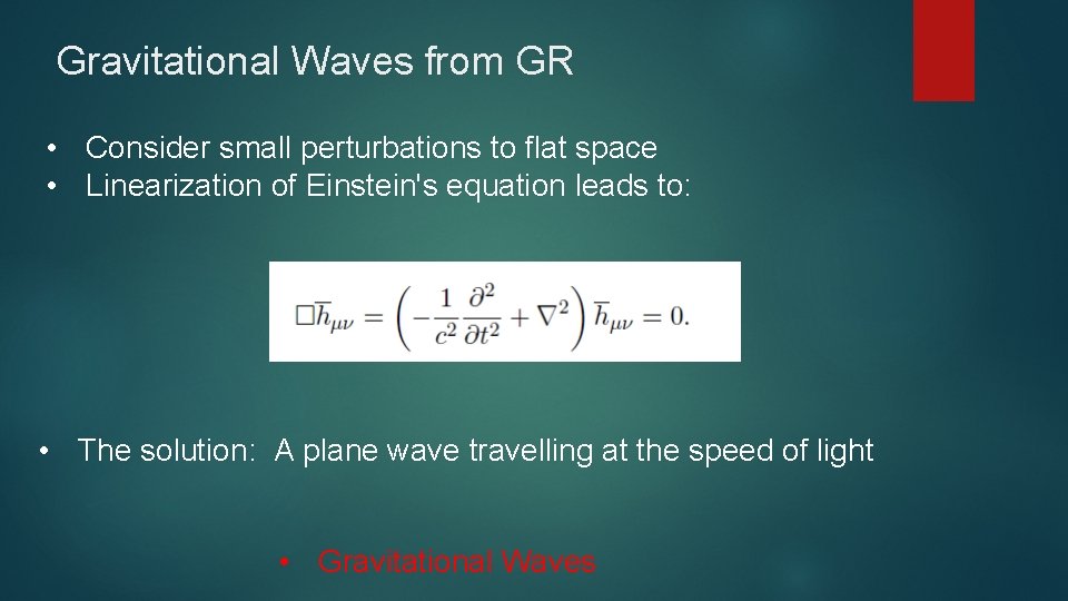
Gravitational Waves from GR • Consider small perturbations to flat space • Linearization of Einstein's equation leads to: • The solution: A plane wave travelling at the speed of light • Gravitational Waves

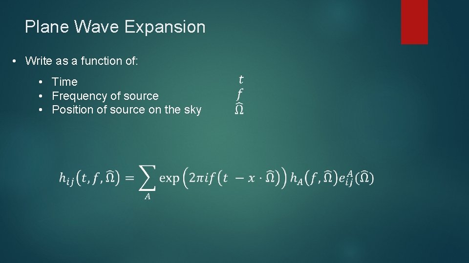
Plane Wave Expansion • Write as a function of: • Time • Frequency of source • Position of source on the sky

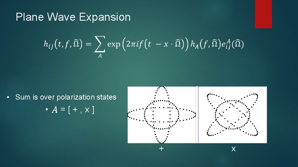
Plane Wave Expansion • Sum is over polarization states • = [ + , x ] + x

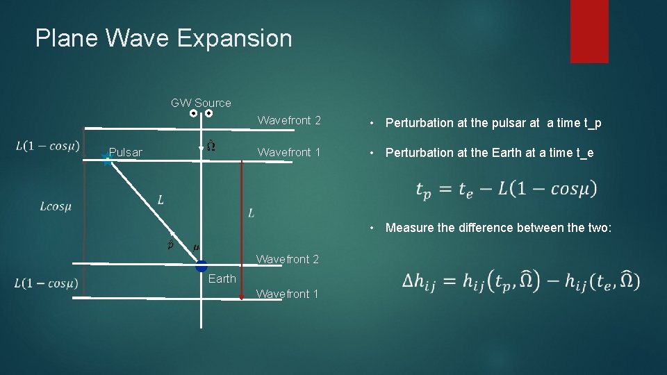
Plane Wave Expansion GW Source Pulsar Wavefront 2 • Perturbation at the pulsar at a time t_p Wavefront 1 • Perturbation at the Earth at a time t_e • Measure the difference between the two: Wavefront 2 Earth Wavefront 1

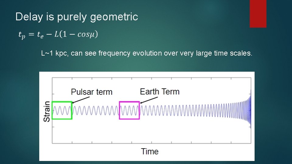
Delay is purely geometric L~1 kpc, can see frequency evolution over very large time scales.

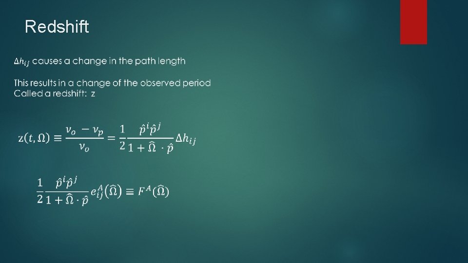
Redshift

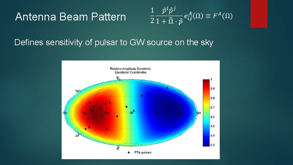
Antenna Beam Pattern Defines sensitivity of pulsar to GW source on the sky

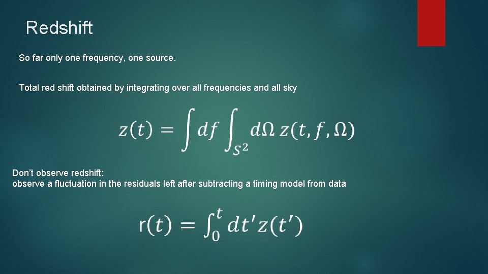
Redshift So far only one frequency, one source. Total red shift obtained by integrating over all frequencies and all sky Don’t observe redshift: observe a fluctuation in the residuals left after subtracting a timing model from data

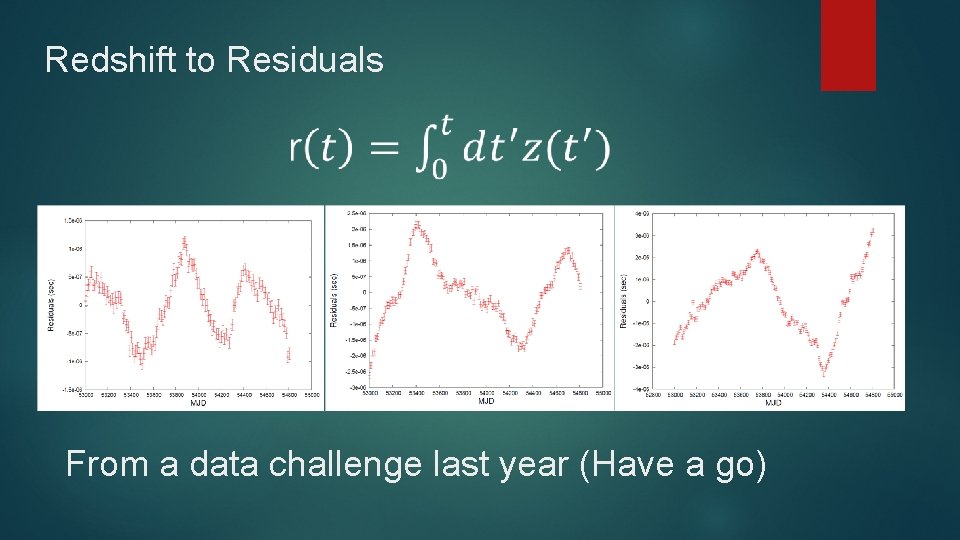
Redshift to Residuals From a data challenge last year (Have a go)

Redshift to Residuals Real pulsars have possible sources of noise other than GWs: Intrinsic red noise Dispersion Measure variations Jitter Need some way to distinguish a gravitational wave background from this ->

The Solution: Signal due to Gravitational Waves is correlated between pulsars other sources of noise (mostly) are not.

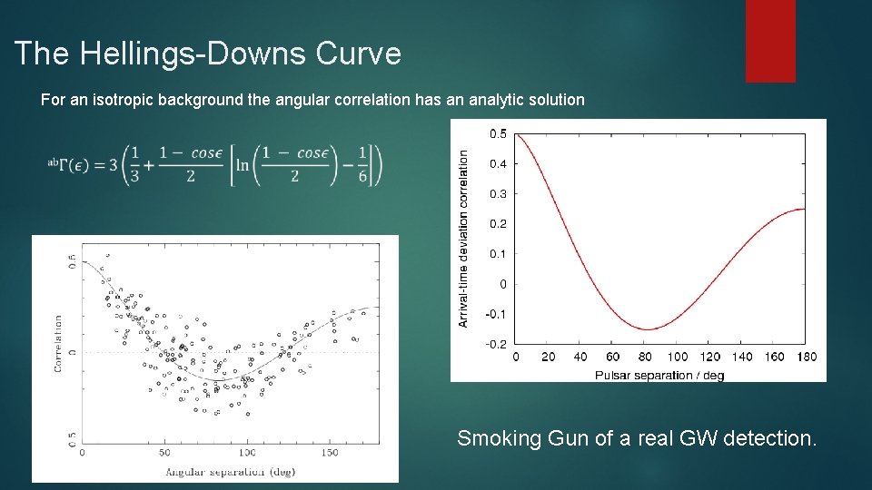
The Hellings-Downs Curve For an isotropic background the angular correlation has an analytic solution Smoking Gun of a real GW detection.

Bayesianism and Frequentism Start at the heart of it. . Asks two different questions: Frequentist: What is the probability of my data, given my model? Assumes model is fixed – data random variable Bayes: What is the probability of my model, given my data? Assumes data is fixed – model is random variable

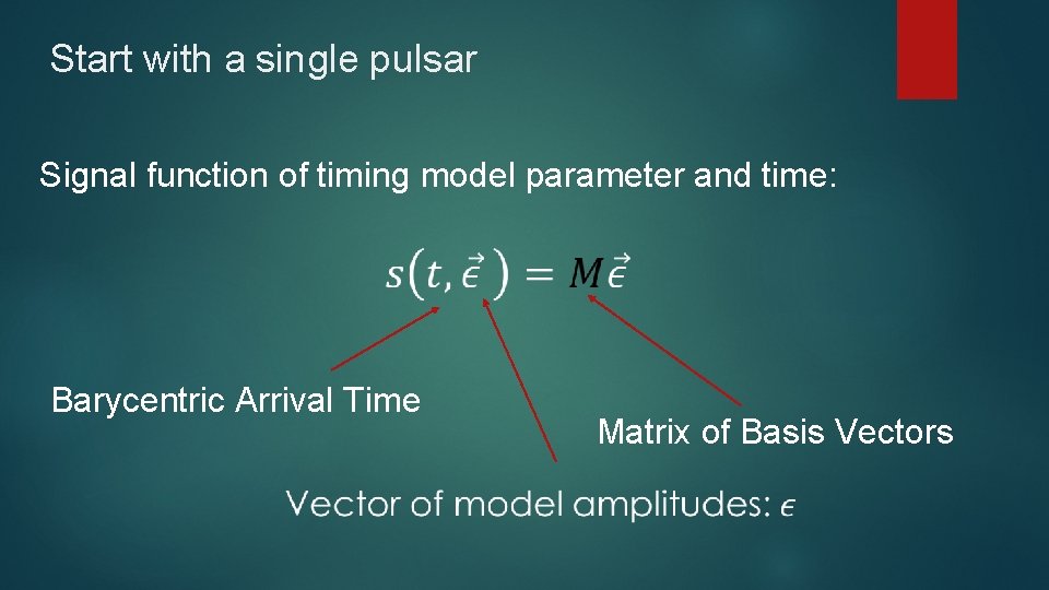
Start with a single pulsar From Earlier this week: • We want to build up a model signal s for the pulsar: • Deterministic signal from timing model

Start with a single pulsar Signal function of timing model parameter and time: Barycentric Arrival Time Matrix of Basis Vectors

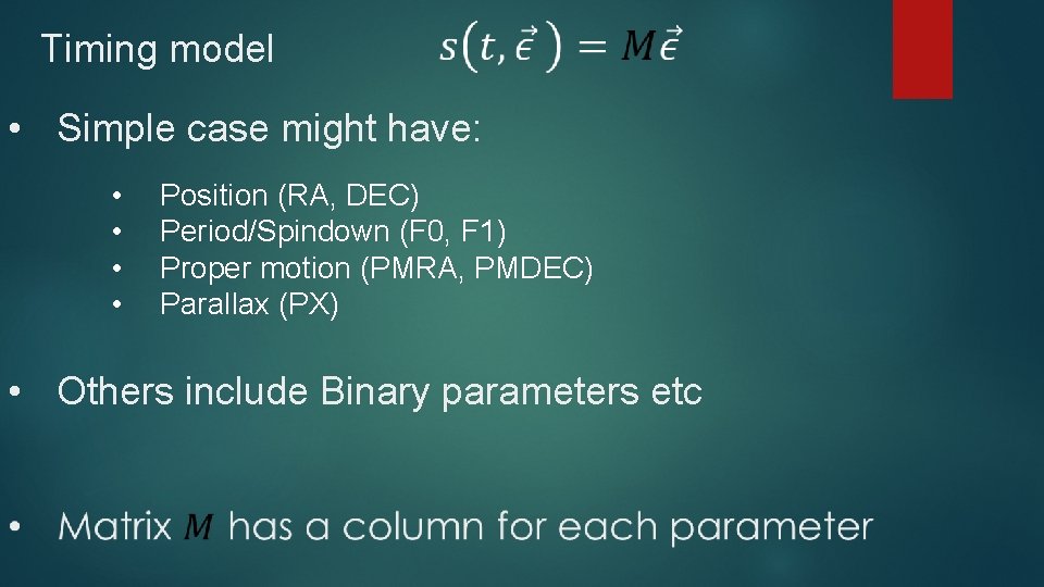
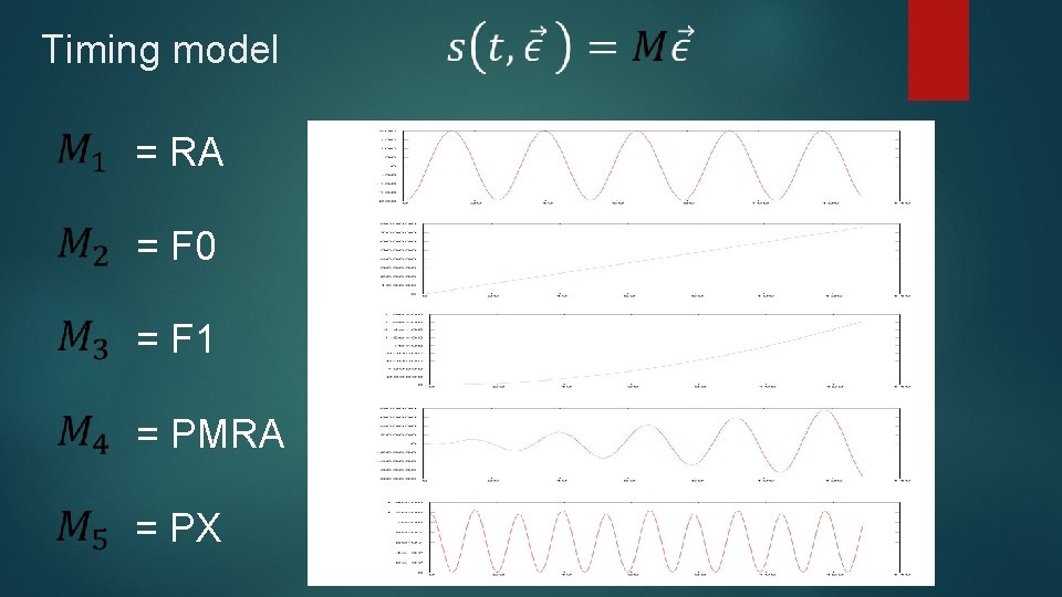
Timing model • Simple case might have: • • Position (RA, DEC) Period/Spindown (F 0, F 1) Proper motion (PMRA, PMDEC) Parallax (PX) • Others include Binary parameters etc

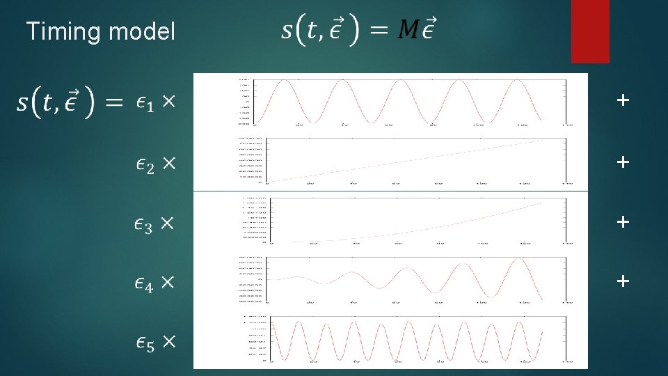
Timing model = RA = F 0 = F 1 = PMRA = PX

Timing model + +

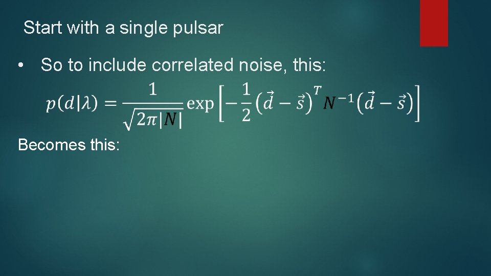
Start with a single pulsar • We Now Have s • What about σ? • Equation above assumes only uncorrelated white noise Almost certainly not true

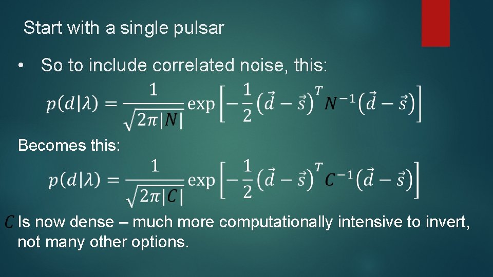
Start with a single pulsar • Rewrite this equation: Is a covariance matrix. Describes the correlations between the residuals . Diagonal = Uncorrelated (as before). Off Diagonal terms imply correlations between times.

Start with a single pulsar • So to include correlated noise, this: Becomes this:

Start with a single pulsar • So to include correlated noise, this: Becomes this: Is now dense – much more computationally intensive to invert, not many other options.

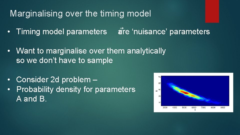
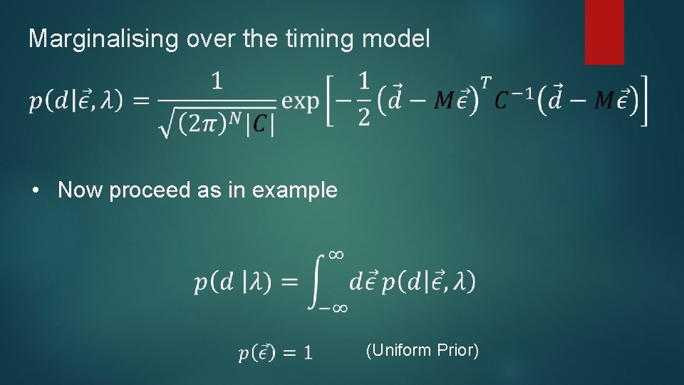
Marginalising over the timing model • Timing model parameters are ‘nuisance’ parameters • Want to marginalise over them analytically so we don’t have to sample • Consider 2 d problem – • Probability density for parameters A and B.

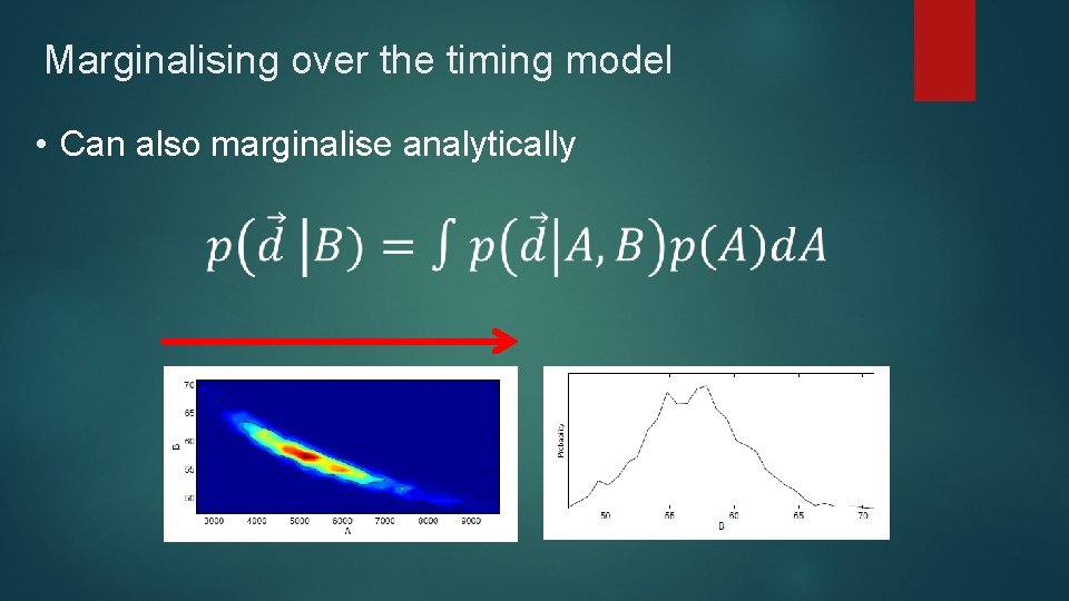
Marginalising over the timing model • Can also marginalise analytically

‘Marginalisation’ Volume Matters

Marginalising over the timing model • Now proceed as in example (Uniform Prior)

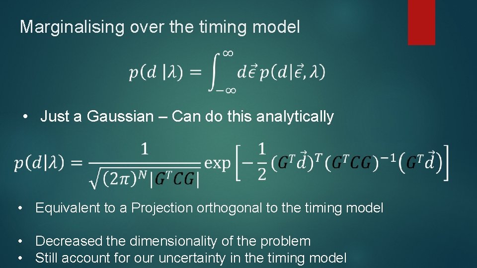
Marginalising over the timing model • Just a Gaussian – Can do this analytically • Equivalent to a Projection orthogonal to the timing model • Decreased the dimensionality of the problem • Still account for our uncertainty in the timing model

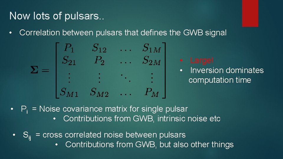
Now lots of pulsars. . • Correlation between pulsars that defines the GWB signal • Large! • Inversion dominates computation time • Pi = Noise covariance matrix for single pulsar • Contributions from GWB, intrinsic noise etc • Sij = cross correlated noise between pulsars • Contributions from GWB, but also other things

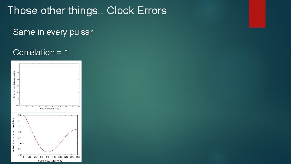
Those other things. . Clock Errors Same in every pulsar Correlation = 1

Those other things. . Planet masses Errors in Planetary Ephemeris -> Error in location of barycentre Orbits 0. 2 -> 164 years Introduces sine wave Period of orbital period Correlated between pulsars Lets you measure mass of planets using pulsars

It all adds up. . Total dimensionality ~ hundreds Weeks of compute time Difficult problem!

Sampling Said we want to calculate P(X |D, M) Non-trivial for non-trivial problems Have to sample from posterior

Markov-Chain Monte-Carlo Markov chain – sequence of state changes that depends only on the most recent states, not the states that preceded them. Simple example (from Wikipedia) Probability of the weather.

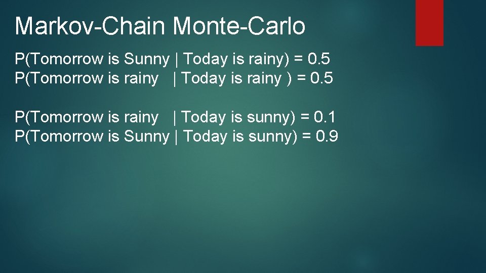
Markov-Chain Monte-Carlo P(Tomorrow is Sunny | Today is rainy) = 0. 5 P(Tomorrow is rainy | Today is rainy ) = 0. 5 P(Tomorrow is rainy | Today is sunny) = 0. 1 P(Tomorrow is Sunny | Today is sunny) = 0. 9

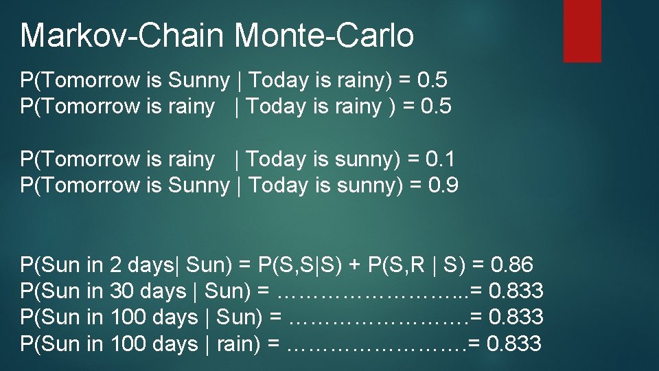
Markov-Chain Monte-Carlo P(Tomorrow is Sunny | Today is rainy) = 0. 5 P(Tomorrow is rainy | Today is rainy ) = 0. 5 P(Tomorrow is rainy | Today is sunny) = 0. 1 P(Tomorrow is Sunny | Today is sunny) = 0. 9 P(Sun in 2 days| Sun) = P(S, S|S) + P(S, R | S) = 0. 86 P(Sun in 30 days | Sun) = …………. . . = 0. 833 P(Sun in 100 days | Sun) = …………. = 0. 833 P(Sun in 100 days | rain) = …………. = 0. 833

Markov-Chain Monte-Carlo Probability of weather tomorrow depends only on the last few days. Forgets about everything previous. Important aspect of all samplers.

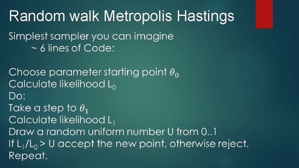
Random walk Metropolis Hastings

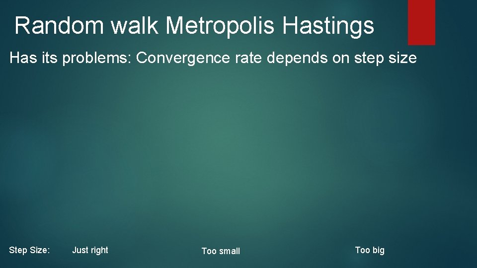
Random walk Metropolis Hastings Has its problems: Convergence rate depends on step size Step Size: Just right Too small Too big

Random walk Metropolis Hastings But will get there eventually Step Size: Just right Too small Too big

Random walk Metropolis Hastings Very poor for multi modal problems: If step size allows jumps between modes, it will be too big within each mode. If step size small enough to explore individual modes, it wont step between them.

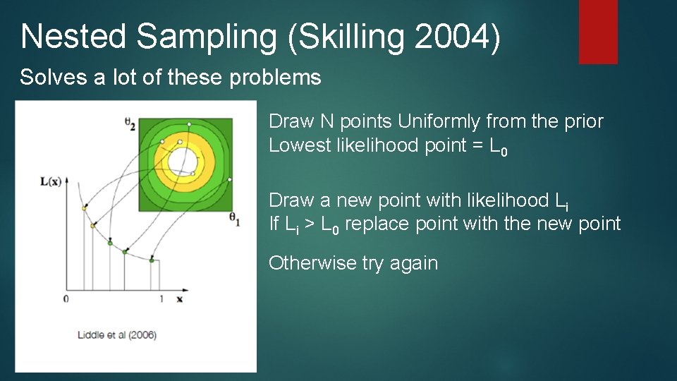
Nested Sampling (Skilling 2004) Solves a lot of these problems Draw N points Uniformly from the prior Lowest likelihood point = L 0 Draw a new point with likelihood Li If Li > L 0 replace point with the new point Otherwise try again

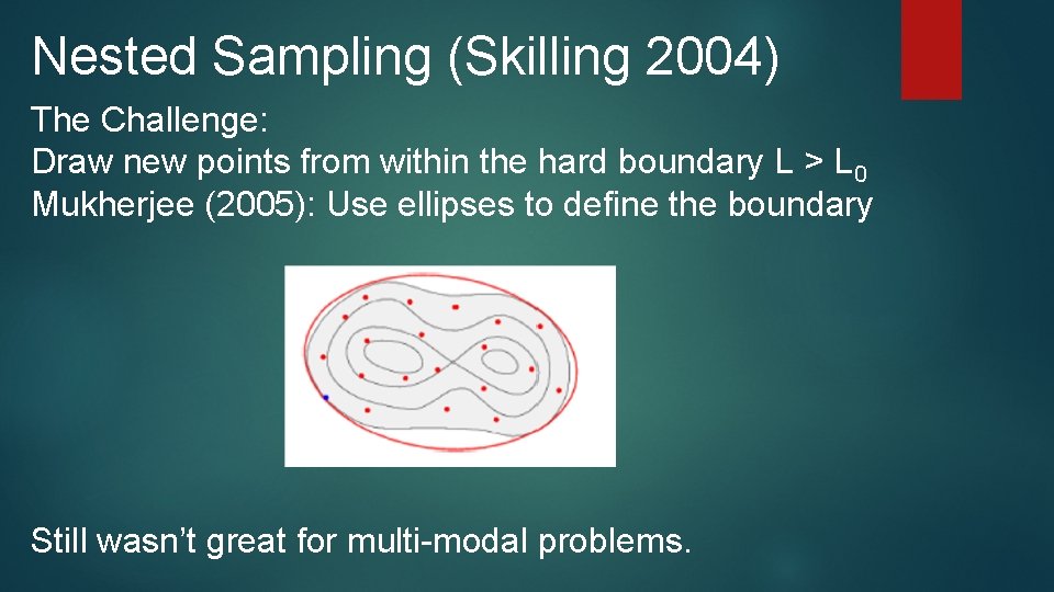
Nested Sampling (Skilling 2004) The Challenge: Draw new points from within the hard boundary L > L 0 Mukherjee (2005): Use ellipses to define the boundary Still wasn’t great for multi-modal problems.

Multi. Nest (Feroz & Hobson 2008) At each iteration: Construct optimal multi-ellipsoidal bound Pick ellipse at random to sample new point

Multi. Nest (Feroz & Hobson 2008) Works great for multi-modal problems:

Polychord (Handley & Hobson 2015) Successor to Multi. Nest. Still uses nested sampling. Works in much higher dimensions (up to ~ 150)

Still a lot to do Modelling Sampling Making Datasets agree… Which is (maybe) why you’re here!