Designing Studies of Medical Tests Farhad Hosseinpanah Obesity

"Designing Studies of Medical Tests" Farhad Hosseinpanah Obesity Research Center Research Institute for Endocrine sciences Shahid Beheshti University of Medical Sciences September 15, 2018 Tehran

Agenda • Introduction • Studies of test reproducibility • Studies of the accuracy of tests

"Development of diagnostic techniques has greatly accelerated but the methodology of diagnostic research lags far behind that for evaluating treatments. "

Introduction

Most designs for studies of medical tests are Descriptive

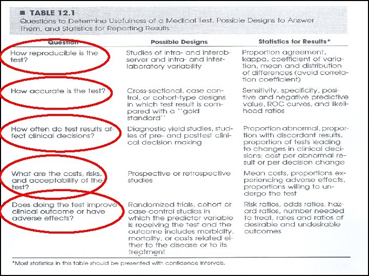
Study of Diagnostic Test: • Causality is generally irrelevant • Main goal is to determine usefulness in clinical practice

Usefulness in clinical practice: • Accuracy • Reproducibility • Feasibility • Effects on clinical decisions and outcomes

Studies of test reproducibility

Precision (or reliability or reproducibility) • The extent that repeated measurements of a phenomenon tend to yield the same results • Precision refers to the lack of random error – Precision ~ 1 / random error

Reliability Measurement Error

Variation in Clinical Data • 1. Biologic Variation= variation in the actual entity being measured – derives from the dynamic nature of physiology, homeostasis and pathophysiology. – within (intra-person) biologic variability and, – between (inter-person) biologic variability

Variation in Clinical Data • 2. Measurement Variation= variation due to the measurement process – inaccuracy of the instrument (instrument error), and/or, – inaccuracy of the person (operator error)

Main sources of error • Subject or biological variability (inter & intra person ) • Observer variability (Inter & Intra observer) • Instrument variability (Within & Between Instrument)

Intraobserver variability • Describes the lack of reproducibility in results when the same observer or laboratory performs the test at different times • A radiologist , same chest radiograph , on two occasions

Interobserver variability • Describes the lack of reproducibility among two or more observers • Two radiologist , same chest radiograph

Important point • Ideally, the only source of variability in a study should be that between study participants.

RCV = 2 Z * (CVA 2 + CVI 2)1/2 ½* Variation in Clinical Data Measurement Variation instrument error operator error CVA Biologic Variation within (intra-person) biologic variability CVA between (inter-person) biologic variability CVI CVG

Reproducibility study • Cross sectional design • Do not require a gold standard • Categorical vs. continuous variables • Main source of error

Reliability indices Mean difference between paired measurements Overall percent agreement Kappa statistic Weighted kappa Coefficient of variation Intraclass coefficient of variation

Categorical variables • Overall percent agreement • Kappa statistic • Weighted kappa Continous variables • Mean difference between paired measurements • Coefficient of variation • Correlation coefficient • Intraclass coefficient of variation

Agreement A perfect standard is not available

Agreement imperfect standard positive New test negative positive a b negative c d overall percent agreement : 100% x (a+d)/(a+b+c+d)

Kappa % observed agreement – % agreement expected by chance 100% – % agreement expected by chance

Imperfect standard new test positive negative total positive 41 3 44 (58. 6%) negative 4 27 31 (41. 4%) total 45 (60%) 30 (40%) 75 (100%) percent observed agreement = 41 + 27 *100 =90. 7% 75

new test positive Imperfect standard positive negative 26. 4 negative total 44 (58. 6%) 31 (41. 4%) 45 (60%) 45 *44 =26. 4% 75 30 (40%) 75 (100%)

Imperfect standard new test positive 26. 4 negative 18. 6 total 45 (60%) negative 17. 6 12. 4 30 (40%) total 44 (58. 6%) 31 (41. 4%) 75 (100%) percent agreement expected by chance = 26. 4 + 12. 4 *100=51. 7% 75

Kappa = % observed agreement – % agreement expected by chance 100% – % agreement expected by chance K= 90. 7% - 51. 7% = 39% = 0. 81 100% - 51. 7% 48. 3%

Level of agreement • > 0. 75 excellent agreement • 0. 4 -0. 75 intermediate • < 0. 4 poor

• Co-efficient of Variation (CV) % – Represents the % variation of a set of measurements around their mean – seful index for comparing the precision of different instruments, individuals and/or laboratories.

Studies of the accuracy of tests

Validity Does the test measure what it is designed to measure?

Validity • Degree to which a measurement process measures what is intended i. e. , accuracy. • Lack of systematic error or bias. • A valid instrument will, on average, be close to the underlying true value. • Assessment of validity requires a “gold standard” (a reference).

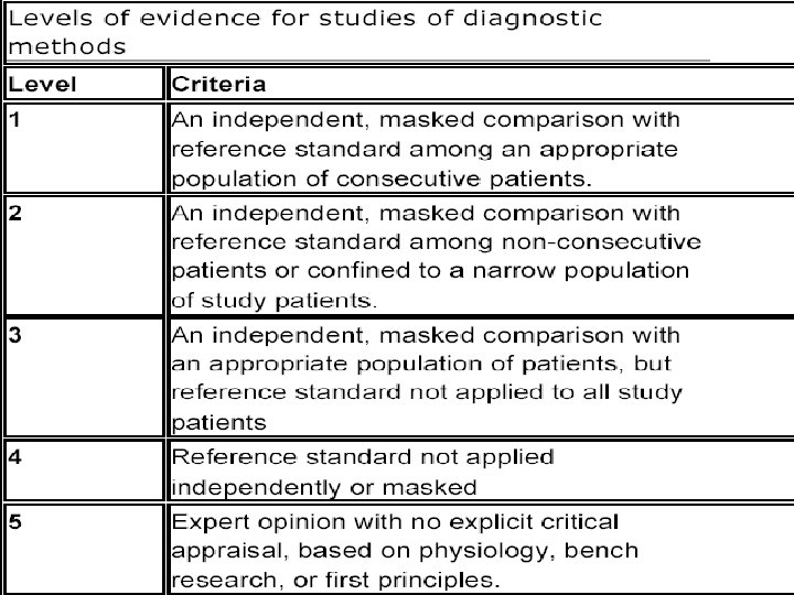
• Different phases of diagnostic studies

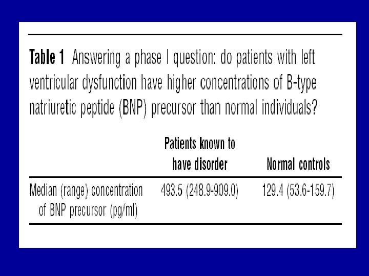
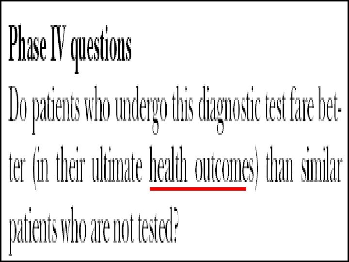
Case-referent approach Phase I questions: Do test results in patients with the target disorder differ from those in normal people?

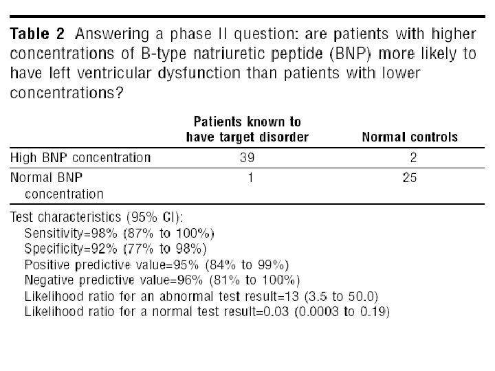
test based enrolment Phase II questions: Are patients with certain test results more likely to have the target disorder than patients with other test results?

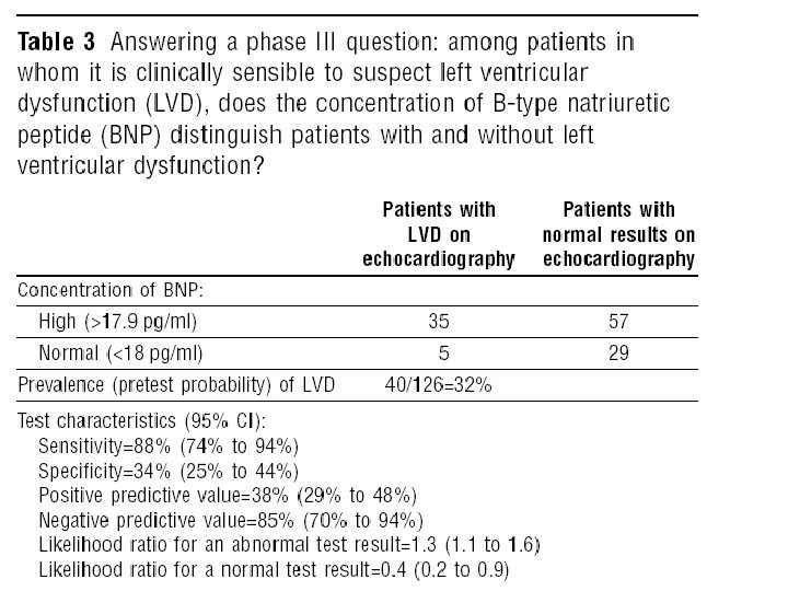
Survey of total study population Phase III questions Does the test result distinguish patients with and without the target disorder among patients in whom it is clinically reasonable to suspect that the disease is present? üMust be prospective üLess clinical contrast üLarger sample size

Validity • Did selection lead to an appropriate spectrum of participants (like those assessed in practice) • What was the gold standard of diagnosis? • Did the results of the test being evaluated influence the decision to perform the reference standard? • Was there a blind comparison between the test and an independent Gold (reference) Standard? • Were the methods for performing the test described in sufficient detail to permit replication?

Spectrum • Participants with the range of common presentations of the target disorder and with commonly confused diagnosis • Florid cases & asymptomatic volunteers only • Spectrum bias • Sensitivity up, specificity up

Spectrum Bias • Spectrum of disease and non disease differs from clinical practice. • Sensitivity depends on spectrum of disease. • Specificity depends on spectrum of non disease or of diseases that might mimic the disease of interest.

Spectrum Bias When disease is skewed toward higher severity than in clinical practice , “sickest of the sick. ” Sensitivity When nondisease is skewed toward greater health, “wellest of the well. ” Specificity

Spectrum Bias • Diagnostic accuracy of low MCV for iron deficiency anemia in the US vs Africa ? • Occult blood for diagnosis of colon cancer in two population with different prevalence of peptic ulcer?

Sensitivity specificity Case control +++++ Hospital practice +++ ++ General practice ++ üSeverity of disease üAlternative diagnosis

Practical point • When you read a paper that tries to measure sensitivity and specificity, think about whether the spectrums of disease and nondisease in the study subjects are similar to those in patients you are likely to see. • As a general rule, the more severe the disease in the patients who have it, the greater the sensitivity, whereas the healthier the “nondiseased” group, the greater the specificity

Gold standard • A different test that is known to give an accurate answer (but that may be more expensive or more invasive than the new test) • A composite of several tests • The result of another medical procedure (such as surgery) • The outcome of a period of follow-up (indicating whether the person develops the condition in question).

Gold standard • 1. Laboratory tests (Infectious & endocrine diseases) • 2. Imaging (DVT, PTE ) • 3. Biopsy (Cancer , vasculitis) • 4. Autopsy (neurologic diseases) • 5. long-term follow-up (SLE , MS)

Independency • The properties of a diagnostic test will be distorted if its result influences whether patients undergo confirmation by the reference standard. • People who are positive on the index test are more likely to get the gold standard, and only those who receive the gold standard are included in the study( Verification bias) • Sensitivity up, specificity down

Ankle swelling and x-ray

Blinding • Those applying and interpreting the reference standard should ideally be unaware of the result of the test. • The pulmonary nodule on CT , and comparison to CXR

Sufficient details • This description should cover all issues that are important in the preparation of the patient (diet, drugs to be avoided, precautions after the test), the performance of the test (technique, possibility of pain), and the analysis and interpretation of its results

Validity indices Sensitivity Specificity PPV NPV Likelihood ratio ROC curve

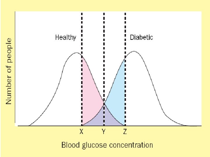
Outcome of diagnostic process • Dichotomous result – diseased or non-diseased • Dichotomous measure – presence or absence of bacteria • Continuous measure – Blood glucose, white cell count, antibody titre – convert to dichotomous result – choice of ‘cut-off’ or ‘normal range’

Biologic Variation of Human Populations • Bimodal curve: distribution with 2 peaks – Relatively easy to separate most of the population into 2 groups (e. g. , ill & not ill; have condition or abnormality & do NOT have condition or abnormality) – Some fall into “gray zone” – may belong to either curve – Most human characteristics are NOT distributed bimodally

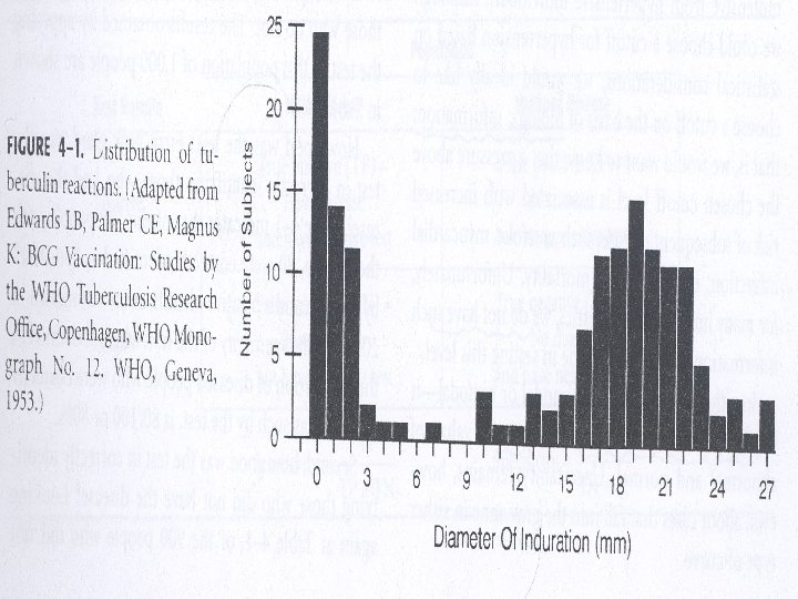
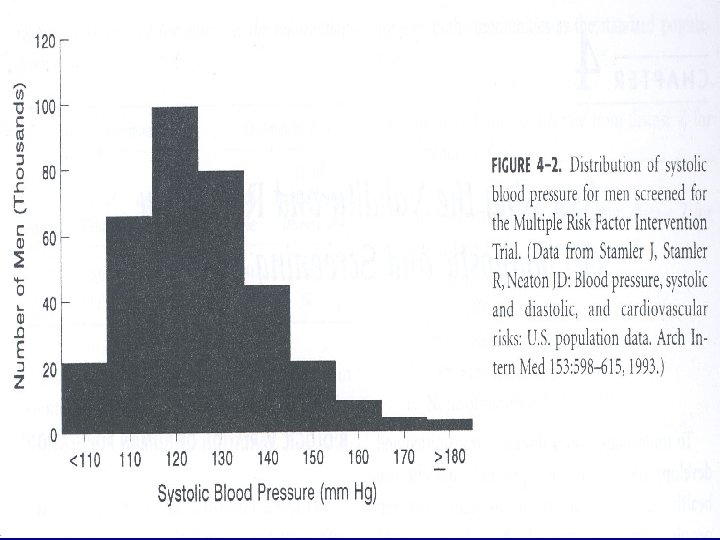
Biologic Variation of Human Populations • Unimodal curve: distribution with 1 peak – Must set a cutoff level to distinguish those with condition & those without condition – Relatively easy to to distinguish the extreme values of abnormal & normal – Uncertainty about those cases in the gray zone

Test result measured on a continuous scale

Gold standard • In any study of diagnosis, the method being evaluated has to be compared to something • The best available test that is used as comparison is called the GOLD STANDARD

2 X 2 tables • To evaluate results of diagnostic studies, we use a 2 X 2 table • By convention, the gold standard goes across the top and the new test goes to the side • The four quadrants of the 2 X 2 represent true positives, false negatives, and true negatives

Information for a dichotomous test Disease Present Absent Positive True positive A False positive B Negative False negative C True negative D Test Result Sensitivity = A / (A+C) Specificity = D / (B+D)

Sensivity and specificity Gold standard + New + test - Sensitivity Specificity

Information for a dichotomous test Disease Present Absent Positive True positive A = 103 False positive B = 16 Negative False negative C = 12 True negative D = 211 Test Result

Information for a dichotomous test Disease Present Absent Positive True positive A = 103 False positive B = 16 Negative False negative C = 12 True negative D = 211 Test Result Sensitivity=103/(103+12)= 89% Specificity=211/(16+211)=93%

Sensitivity and specificity Limitations: • we don’t know who has the disease before the test ! Otherwise we wouldn’t need to order the diagnostic test.

Sensitivity & Specificity of Tests Limitations: • Demand only 2 test results: + or -. Hence all test data cannot be used, but must be collapsed by a “cut-point”. • The “cut-point” can be reset and sen. & spec. recalculated. • Plotting the results of several “cut-points” provides an ROC curve that reveals the overall quality of a test.

Results for a Typical Diagnostic Test Illustrating Overlap Between Disease (D+) and Non-disease (D-) Populations = FP Cut -point = FN D - D + TN T- TP T+ Diagnostic test result (continuous)

Example of a Perfectly Sensitive Test = FP Cut -point D- D + TN T- TP T+ Diagnostic test result

Tests with High Sensitivity • perfectly sensitive test (Se = 100%), all diseased patients are test positive (no FN’s) • all test negative patients are disease free (TNs) but usually many FPs exist. • highly sensitive tests are used to rule-out disease - if the test is negative you can be confident that disease is absent (FN results are rare!). • highly sensitive tests do not tell you if disease is present, because they provides no information regarding FP’s (see Sp). • Sn. Nout = if a sign, symptom or other diagnostic tests has a sufficiently high Sensitivity, a Negative result rules out disease.

Tests with High Sensitivity • Three clinical scenarios where high sensitivity test should be used: – 1) Early stages of a diagnostic work-up. • large number of potential diseases are being considered. • a negative result indicates a particular disease can be dropped (i. e. , ruled out). – 2) Important penalty for missing a disease. • Examples - TB, syphilis - dangerous but treatable conditions. • don’t want to miss cases, hence avoid false negative results – 3) Screening tests. • the probability of disease is relatively low (i. e. , low prevalence) • want to find as many asymptomatic cases as possible (incr. yield)

Table 1. Examples of Tests with High Sensitivities Disease/Condition Test Sensitivity Duodenal ulcer History of ulcer, 50+ yrs, pain relieved by eating or pain after eating 95% Favourable prognosis following non-traumatic coma Corneal reflex 92% High intracranial pressure Absence of spont. pulsation of retinal veins 100% Deep vein thrombosis Positive to impedance plethysmography and/or fibrinogen leg scanning 92% Pancreatic cancer Endoscopic retrograde cholangio- pancreatography (ERCP) 95%

Example of a Perfectly Specific Test = FN Cut -point D - D + TN TDiagnostic test result TP T+

Tests with High Specificity • perfectly specific test (Sp = 100%), all nondiseased patients test negative (no FP’s) • all test positive patients have disease (TPs) but usually sizeable number of FNs • highly specific tests are used to rule-in disease - if the test is positive you can be confident that disease is present (FPs are rare). • highly specific tests do not tell you if disease is absent, because Sp provides no information regarding FNs (see Se). • Sp. Pin = if a sign, symptom or other diagnostic tests has a sufficiently high Specificity, a Positive result rules in disease.

Tests with High Specificity • Clinical scenarios when high specificity tests should be used: – 1) To rule-in a diagnosis suggested by other tests • specific tests are therefore used at the end of a workup to rule-in a final diagnosis e. g. , biopsy, culture, CT scan. – 2) False positive tests results can harm patient • want to be absolutely sure that disease is present. • example, the confirmation of HIV positive status or the confirmation of cancer prior to chemotherapy.

Table 2. Examples of Tests with High Specificities Disease/Condition Test Specificity Alcohol dependency Yes to 3 or more of the 4 CAGE questions 99. 7% Iron-deficiency anemia Serum ferritin 90% Deep vein thrombosis Negative to impedance plethysmography and/or fibrinogen leg scanning 92% Pancreatic cancer Endoscopic retrograde cholangio- pancreatography (ERCP) 97% Breast cancer Fine needle aspirate 98% Strep throat Pharyngeal gram stain 96%

Trade-off Between Se and Sp: Lowering the Test Cut-point Increases Se but Decreases Sp = FP Cut -point = FN D - D + TN TP TDiagnostic test result T+

Using sensitivity and specificity • As a consequence, you tend to believe a sensitive test when it is negative (rules out the disease) • You tend to believe a specific test when it is positive (rules in the disease) • Way to remember: – Sensitive rules out (SNOUT) – Specific rules in (SPIN)

Information for a dichotomous test Disease Present Absent Positive True positive A = 103 False positive B = 16 Negative False negative C = 12 True negative D = 211 Test Result

Information for a dichotomous test Disease Present Absent True positive Positive A False positive B False negative Negative C True negative D Test Result Sensitivity = A / (A+C) Specificity = D / (B+D) sen * prevalence PPV = A / (A+B) = (sen*prev)+ (1 -spec)*(1 -prev) NPV = D / (C+D) = Spec*(1 -prev) (1 -sen)*prev+spec*(1 -prev)

Information for a dichotomous test Disease Present Absent Positive True positive A = 103 False positive B = 16 Negative False negative C = 12 True negative D = 211 Test Result Sensitivity=103/(103+12)=89% Specificity=211/(16+211)=93% PPV = 103 / (103+16) = 86% NPV = 211 / (12+211) = 94%

Pos and Neg Predictive Value Gold standard + New + + PV TP/TP+FP test - - PV TN/TP+FN Sensitivity Specificity

Using predictive values • Tell you whether you should believe your test results: very clinically useful!! • Unlike sens and spec, predictive values are dependent upon the test and the population that you are testing • While sensitivity and specificity are constants, Predictive Values change depending upon who you are testing

Predictive values • Limitation: predictive values are dependent on the fixed prevalence (pretest probability) of disease in the studied population. If the pretest probability of the disease is equal to prevalence of disease then the post test probability of disease will be equal to PPV (e. g in screening)

Example: low prevalence 1% of people have disease out of 1, 000 tested + + PV + 99 8. 3% New - 1 891 - PV 99. 9% Sensitivity Specificity 90%

Example 2: High prevalence 99% of people have disease out of 1, 000 tested + + PV + 891 1 99. 9% New - 99 9 - PV 8. 3% Sensitivity Specificity 90%

Example 3: Medium prevalence 50% of people have disease out of 1, 000 tested + + PV + 450 50 90% New - 50 450 - PV 90% Sensitivity Specificity 90%

Sensitivity 80% , specificity 90% Pretest probability 1% 10% 50% 90% PPV 7. 5% 47. 1% 88. 9% 98. 6% NPV 99. 8% 97. 6% 81. 8% 33. 3%

The PVP and PVN as a Function of Prevalence for a Typical Diagnostic Test Predictive Value 1. 0. 80 PV+ . 60. 40 PV- . 20 0 . 20 . 40 . 60 . 80 1. 0 Prevalence or Prior probability

• As prevalence falls, positive predictive value must fall along with it, and negative predictive value must rise. Conversely, as prevalence increases, positive predictive value will increase and negative predictive value will fall.

Likelihood ratio • Likelihood ratio = the likelihood of a test result in patients with the disease / the likelihood of a test result in patients without the disease – LR(+) = sensitivity/(1 -specificity) – LR(-) = (1 -sensitivity)/specificity

Likelihood ratios • Another way of looking at whether you should believe a test • Compares the odds of having the disease before the test and the odds of having the disease after the test • Based on the ratio of true positives (or negative) to false positive (or negatives) • Larger the likelihood ratio, better the test

Information for a dichotomous test Disease Present Absent Positive True positive A = 103 False positive B = 16 Negative False negative C = 12 True negative D = 211 Test Result

Information for a dichotomous test Disease Present Absent Positive True positive A False positive B Negative False negative C True negative D Test Result Sensitivity = A / (A+C) Specificity = D / (B+D) PPV = A / (A+B) NPV = D / (C+D) A /(A+C) LR(+) = = sn / (1 -sp) B / (B+D) C /(A+C) LR(-) = = (1 -sn) / sp D / (B+D)

Information for a dichotomous test Disease Present Absent Positive True positive A = 103 Negative False negative True negative C = 12 D = 211 Test Result False positive B = 16 Sensitivity=103/(103+12)=89% A /(A+C) LR(+) = = sn / (1 -sp)=12. 7 B / (B+D) Specificity=211/(16+211)=93% PPV = 103 / (103+16) = 86% NPV = 211 / (12+211) = 94% C /(A+C) LR(-) = = (1 -sn) / sp=0. 11 D / (B+D)

LR Interpretation > 10 Large and often conclusive increase in the likelihood of disease 510 Moderate increase in the likelihood of disease 2 -5 Small increase in the likelihood of disease 1 -2 Minimal increase in the likelihood of disease

LR INTERPRETATION 1 No change in the likelihood of disease 0. 5 1. 0 Minimal decrease in the likelihood of disease 0. 2 0. 5 Small decrease in the likelihood of disease 0. 1 - Moderate decrease in the likelihood 0. 2 of disease Large and often conclusive decrease < 0. 1 in the likelihood of disease

Seven standards Standard 1: Spectrum composition Standard 2: Pertinent subgroups Standard 3: Avoidance of workup bias Standard 4: Avoidance of review bias Standard 5: Precision of results for test accuracy Standard 6: Presentation of indeterminate test results Standard 7: Test reproducibility