Designing Efficient Cascaded Classifiers Tradeoff between Accuracy and

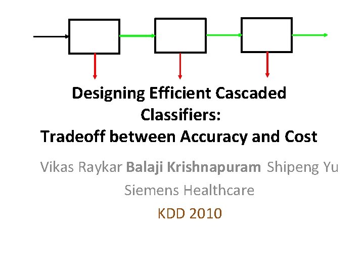
Designing Efficient Cascaded Classifiers: Tradeoff between Accuracy and Cost Vikas Raykar Balaji Krishnapuram Shipeng Yu Siemens Healthcare KDD 2010

Features incur a cost • • Features are acquired on demand. A set of features can be acquired as a group. Each feature group incurs a certain cost. Acquisition cost can be either – Computational | fast detectors – Financial | expensive medical tests – Human discomfort | biopsy

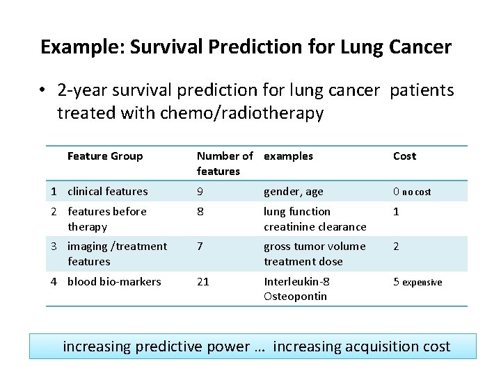
Example: Survival Prediction for Lung Cancer • 2 -year survival prediction for lung cancer patients treated with chemo/radiotherapy Feature Group Number of examples features Cost 1 clinical features 9 gender, age 0 no cost 2 features before therapy 8 lung function creatinine clearance 1 3 imaging /treatment features 7 gross tumor volume treatment dose 2 4 blood bio-markers 21 Interleukin-8 Osteopontin 5 expensive increasing predictive power … increasing acquisition cost

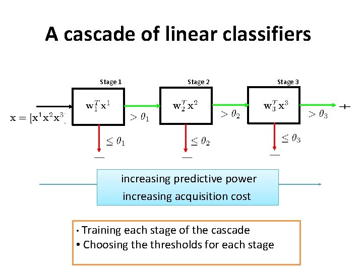
A cascade of linear classifiers Stage 1 Stage 2 increasing predictive power increasing acquisition cost • Training each stage of the cascade • Choosing the thresholds for each stage Stage 3

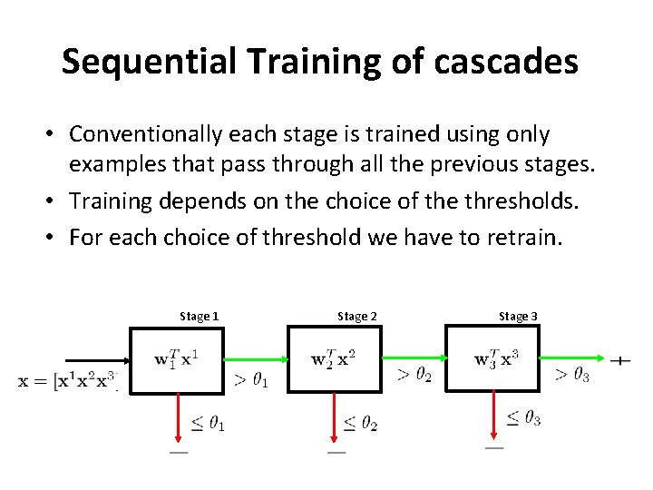
Sequential Training of cascades • Conventionally each stage is trained using only examples that pass through all the previous stages. • Training depends on the choice of the thresholds. • For each choice of threshold we have to retrain. Stage 1 Stage 2 Stage 3

Contributions of this paper • Joint training of all stages of the cascade. – Notion of probabilistic soft cascades • A knob to control the tradeoff between accuracy vs cost – Modeling the expected feature cost • Decoupling the classifier training and threshold selection. – Post-selection of thresholds

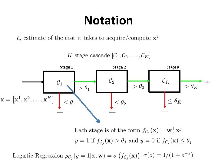
Notation Stage 1 Stage 2 Stage K

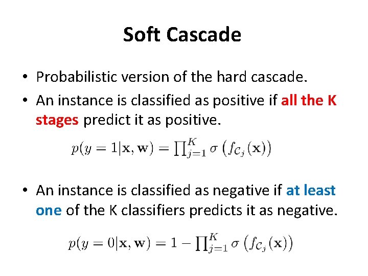
Soft Cascade • Probabilistic version of the hard cascade. • An instance is classified as positive if all the K stages predict it as positive. • An instance is classified as negative if at least one of the K classifiers predicts it as negative.

Some properties of soft cascades • Sequential ordering of the cascade is not important. • Order definitely matters during testing. • A device to ease the training process. • We use a maximum a-posteriori (MAP) estimate with Laplace prior on the weights.

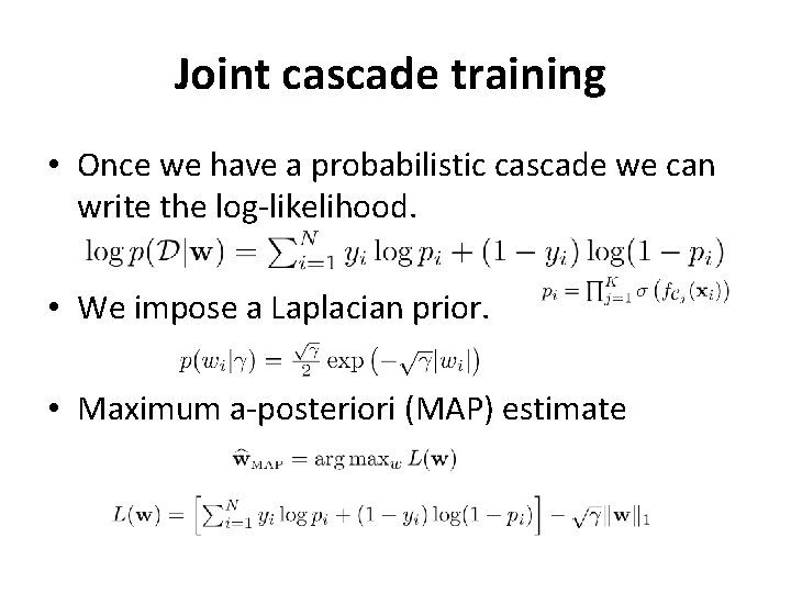
Joint cascade training • Once we have a probabilistic cascade we can write the log-likelihood. • We impose a Laplacian prior. • Maximum a-posteriori (MAP) estimate

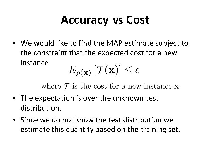
Accuracy vs Cost • We would like to find the MAP estimate subject to the constraint that the expected cost for a new instance • The expectation is over the unknown test distribution. • Since we do not know the test distribution we estimate this quantity based on the training set.

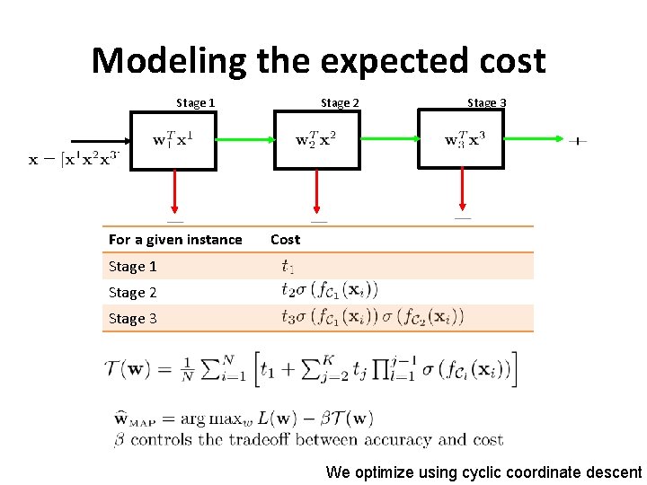
Modeling the expected cost Stage 1 For a given instance Stage 2 Stage 3 Cost Stage 1 Stage 2 Stage 3 We optimize using cyclic coordinate descent

Experiments • Medical Datasets – Personalized medicine • Survival prediction for lung cancer • Tumor response prediction for rectal cancer – Computer aided diagnosis for lung cancer

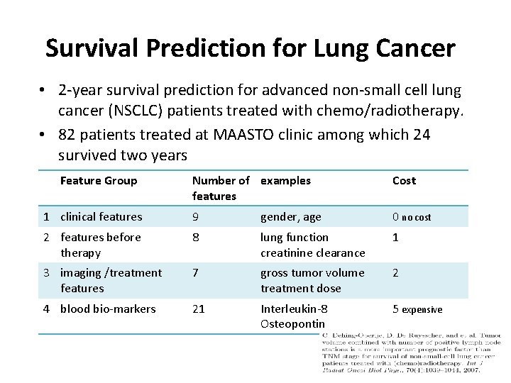
Survival Prediction for Lung Cancer • 2 -year survival prediction for advanced non-small cell lung cancer (NSCLC) patients treated with chemo/radiotherapy. • 82 patients treated at MAASTO clinic among which 24 survived two years Feature Group Number of examples features Cost 1 clinical features 9 gender, age 0 no cost 2 features before therapy 8 lung function creatinine clearance 1 3 imaging /treatment features 7 gross tumor volume treatment dose 2 4 blood bio-markers 21 Interleukin-8 Osteopontin 5 expensive

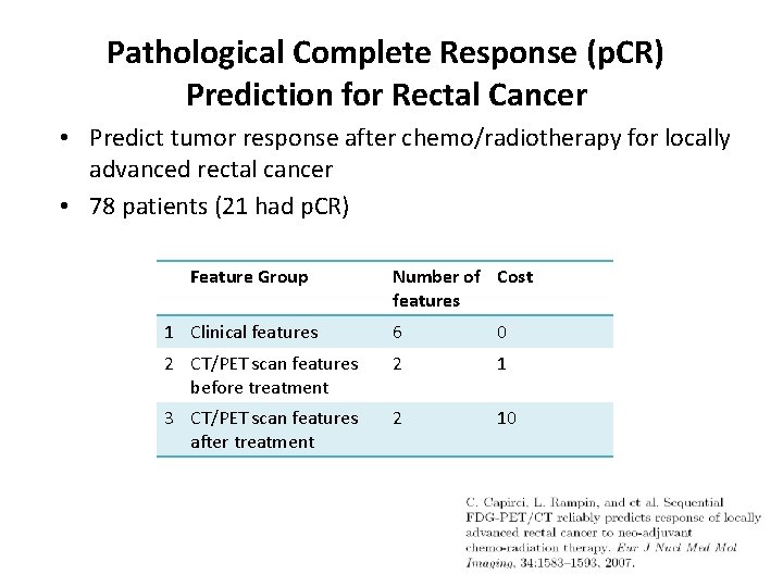
Pathological Complete Response (p. CR) Prediction for Rectal Cancer • Predict tumor response after chemo/radiotherapy for locally advanced rectal cancer • 78 patients (21 had p. CR) Feature Group Number of Cost features 1 Clinical features 6 0 2 CT/PET scan features before treatment 2 1 3 CT/PET scan features after treatment 2 10

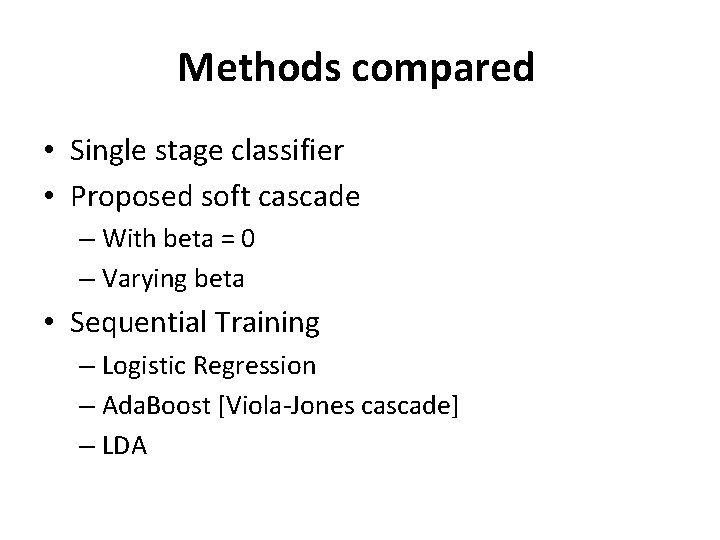
Methods compared • Single stage classifier • Proposed soft cascade – With beta = 0 – Varying beta • Sequential Training – Logistic Regression – Ada. Boost [Viola-Jones cascade] – LDA

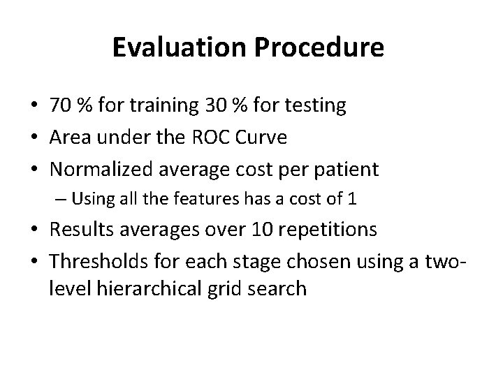
Evaluation Procedure • 70 % for training 30 % for testing • Area under the ROC Curve • Normalized average cost per patient – Using all the features has a cost of 1 • Results averages over 10 repetitions • Thresholds for each stage chosen using a twolevel hierarchical grid search

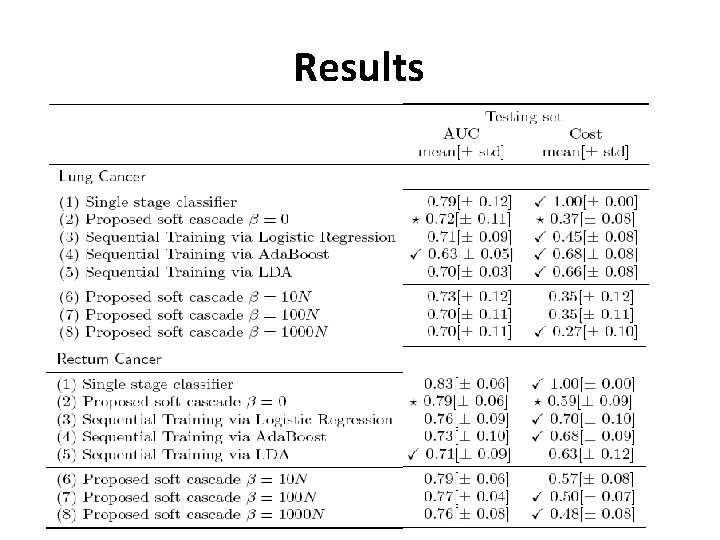
Results

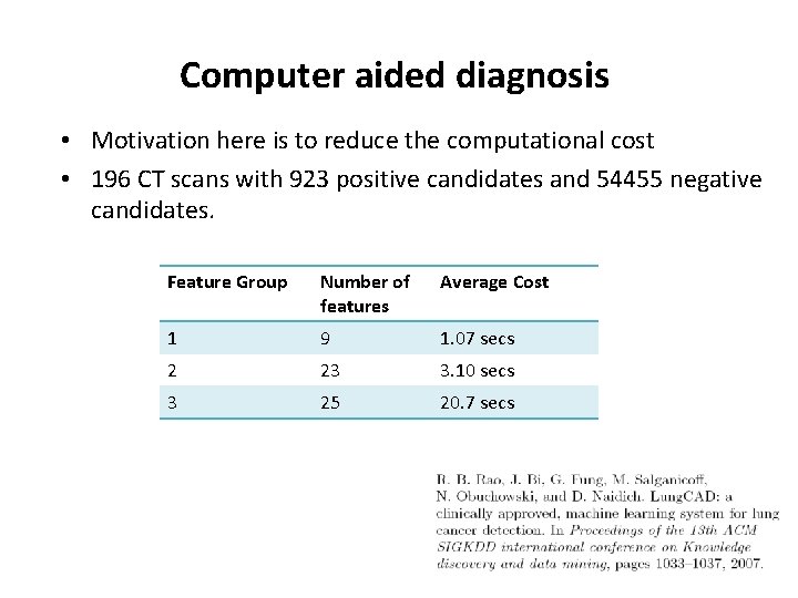
Computer aided diagnosis • Motivation here is to reduce the computational cost • 196 CT scans with 923 positive candidates and 54455 negative candidates. Feature Group Number of features Average Cost 1 9 1. 07 secs 2 23 3. 10 secs 3 25 20. 7 secs

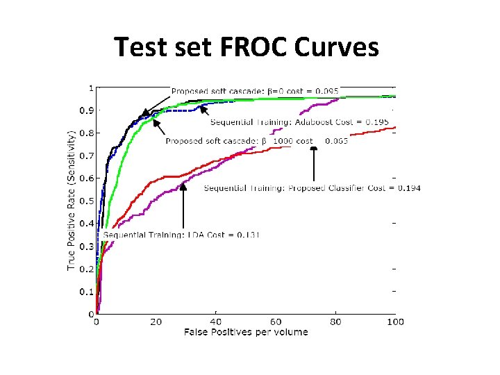
Test set FROC Curves

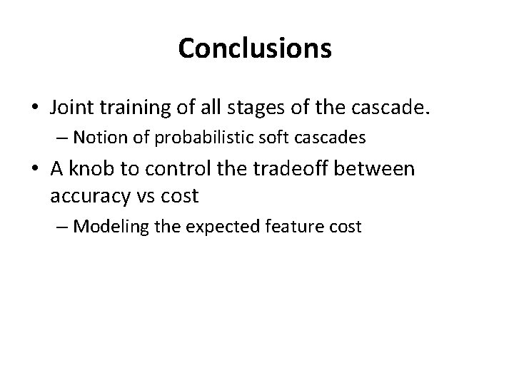
Conclusions • Joint training of all stages of the cascade. – Notion of probabilistic soft cascades • A knob to control the tradeoff between accuracy vs cost – Modeling the expected feature cost

Related work

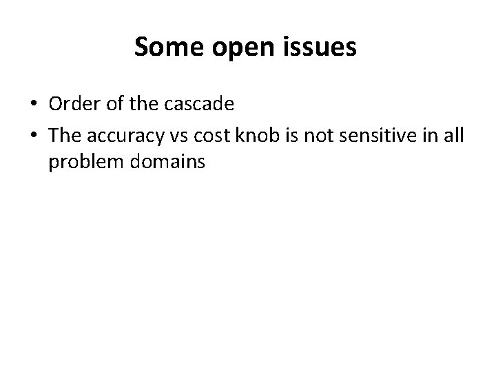
Some open issues • Order of the cascade • The accuracy vs cost knob is not sensitive in all problem domains