Design of Engineering Experiments Part 2 Basic Statistical

Design of Engineering Experiments Part 2 – Basic Statistical Concepts • Simple comparative experiments – The hypothesis testing framework – The two-sample t-test – Checking assumptions, validity • Comparing more that two factor levels…the analysis of variance – – ANOVA decomposition of total variability Statistical testing & analysis Checking assumptions, model validity Post-ANOVA testing of means • Sample size determination DOX 6 E Montgomery 1

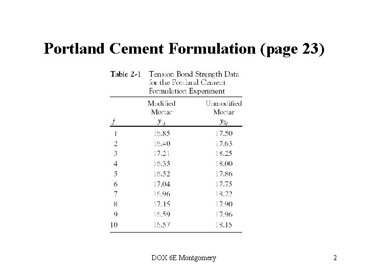
Portland Cement Formulation (page 23) DOX 6 E Montgomery 2

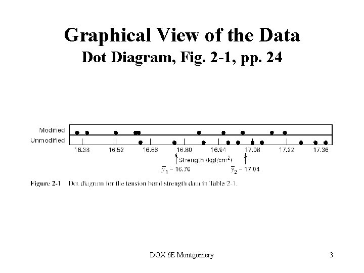
Graphical View of the Data Dot Diagram, Fig. 2 -1, pp. 24 DOX 6 E Montgomery 3

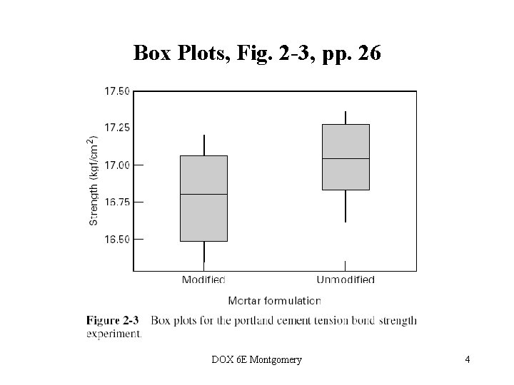
Box Plots, Fig. 2 -3, pp. 26 DOX 6 E Montgomery 4

The Hypothesis Testing Framework • Statistical hypothesis testing is a useful framework for many experimental situations • Origins of the methodology date from the early 1900 s • We will use a procedure known as the twosample t-test DOX 6 E Montgomery 5

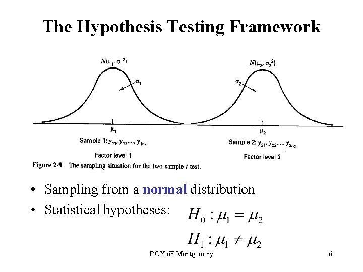
The Hypothesis Testing Framework • Sampling from a normal distribution • Statistical hypotheses: DOX 6 E Montgomery 6

Estimation of Parameters DOX 6 E Montgomery 7

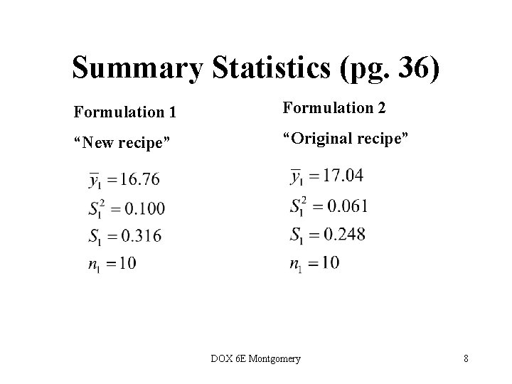
Summary Statistics (pg. 36) Formulation 1 Formulation 2 “New recipe” “Original recipe” DOX 6 E Montgomery 8

How the Two-Sample t-Test Works: DOX 6 E Montgomery 9

How the Two-Sample t-Test Works: DOX 6 E Montgomery 10

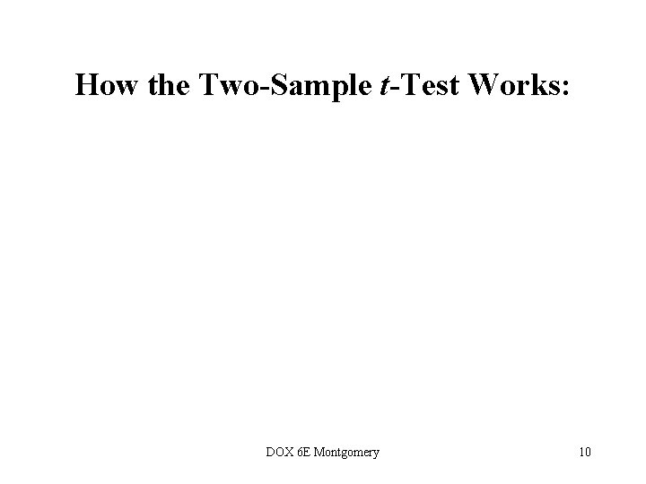
How the Two-Sample t-Test Works: • Values of t 0 that are near zero are consistent with the null hypothesis • Values of t 0 that are very different from zero are consistent with the alternative hypothesis • t 0 is a “distance” measure-how far apart the averages are expressed in standard deviation units • Notice the interpretation of t 0 as a signal-to-noise ratio DOX 6 E Montgomery 11

The Two-Sample (Pooled) t-Test DOX 6 E Montgomery 12

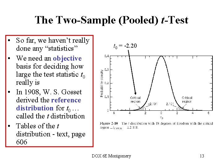
The Two-Sample (Pooled) t-Test • So far, we haven’t really done any “statistics” • We need an objective basis for deciding how large the test statistic t 0 really is • In 1908, W. S. Gosset derived the reference distribution for t 0 … called the t distribution • Tables of the t distribution - text, page 606 t 0 = -2. 20 DOX 6 E Montgomery 13

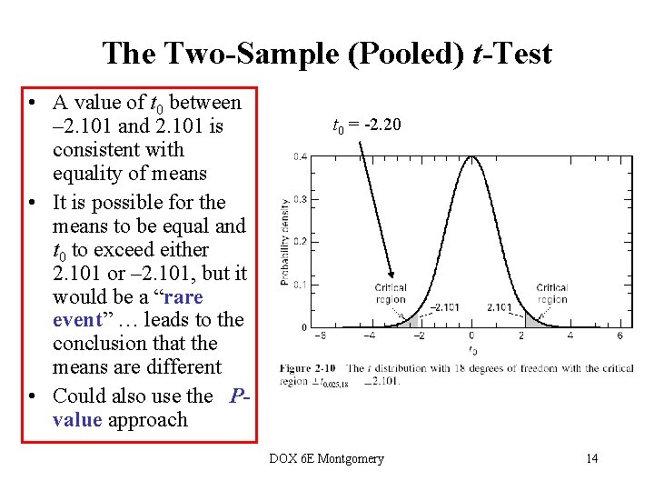
The Two-Sample (Pooled) t-Test • A value of t 0 between – 2. 101 and 2. 101 is consistent with equality of means • It is possible for the means to be equal and t 0 to exceed either 2. 101 or – 2. 101, but it would be a “rare event” … leads to the conclusion that the means are different • Could also use the Pvalue approach t 0 = -2. 20 DOX 6 E Montgomery 14

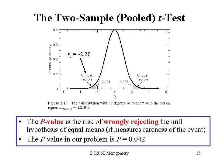
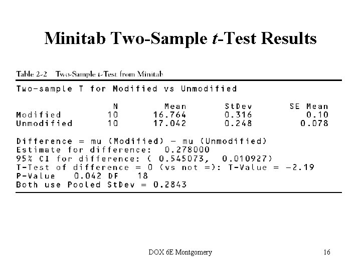
The Two-Sample (Pooled) t-Test t 0 = -2. 20 • The P-value is the risk of wrongly rejecting the null hypothesis of equal means (it measures rareness of the event) • The P-value in our problem is P = 0. 042 DOX 6 E Montgomery 15

Minitab Two-Sample t-Test Results DOX 6 E Montgomery 16

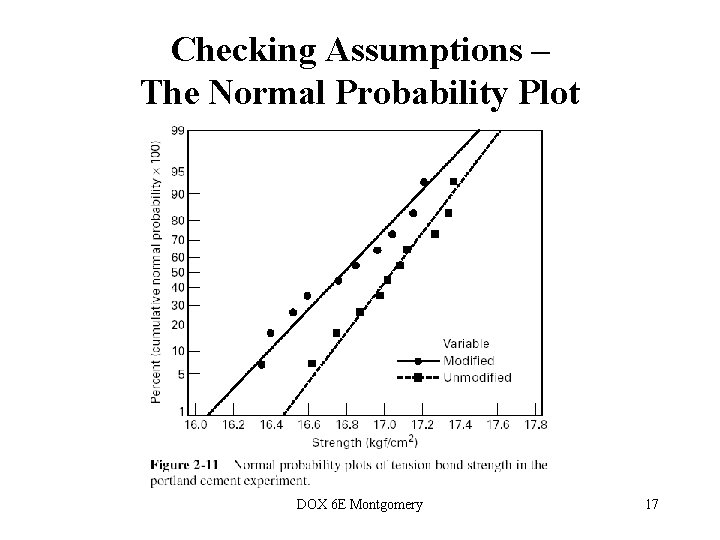
Checking Assumptions – The Normal Probability Plot DOX 6 E Montgomery 17

Importance of the t-Test • Provides an objective framework for simple comparative experiments • Could be used to test all relevant hypotheses in a two-level factorial design, because all of these hypotheses involve the mean response at one “side” of the cube versus the mean response at the opposite “side” of the cube DOX 6 E Montgomery 18

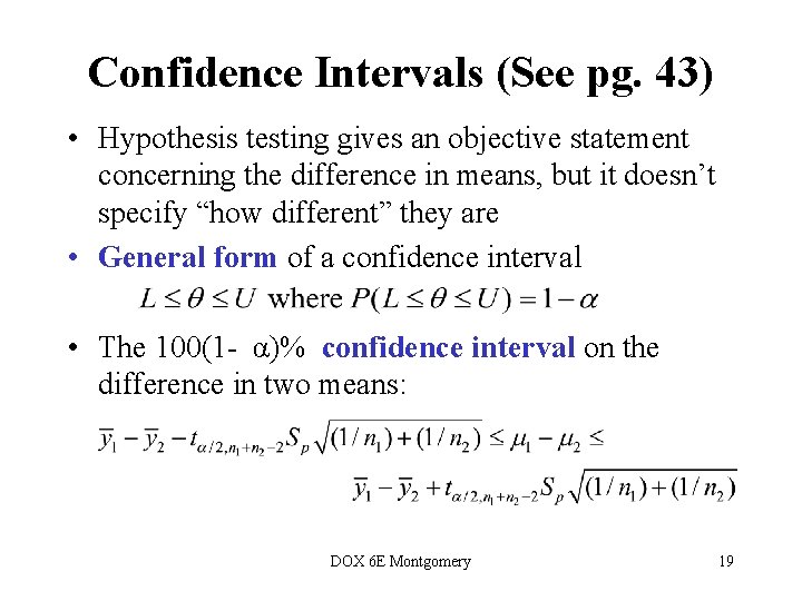
Confidence Intervals (See pg. 43) • Hypothesis testing gives an objective statement concerning the difference in means, but it doesn’t specify “how different” they are • General form of a confidence interval • The 100(1 - α)% confidence interval on the difference in two means: DOX 6 E Montgomery 19

What If There Are More Than Two Factor Levels? • The t-test does not directly apply • There are lots of practical situations where there are either more than two levels of interest, or there are several factors of simultaneous interest • The analysis of variance (ANOVA) is the appropriate analysis “engine” for these types of experiments – Chapter 3, textbook • The ANOVA was developed by Fisher in the early 1920 s, and initially applied to agricultural experiments • Used extensively today for industrial experiments DOX 6 E Montgomery 20

An Example (See pg. 60) • An engineer is interested in investigating the relationship between the RF power setting and the etch rate for this tool. The objective of an experiment like this is to model the relationship between etch rate and RF power, and to specify the power setting that will give a desired target etch rate. • The response variable is etch rate. • She is interested in a particular gas (C 2 F 6) and gap (0. 80 cm), and wants to test four levels of RF power: 160 W, 180 W, 200 W, and 220 W. She decided to test five wafers at each level of RF power. • The experimenter chooses 4 levels of RF power 160 W, 180 W, 200 W, and 220 W • The experiment is replicated 5 times – runs made in random order DOX 6 E Montgomery 21

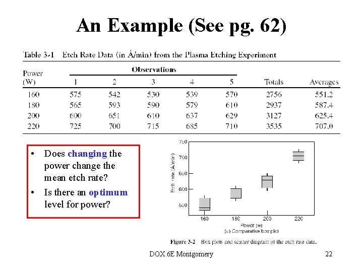
An Example (See pg. 62) • Does changing the power change the mean etch rate? • Is there an optimum level for power? DOX 6 E Montgomery 22

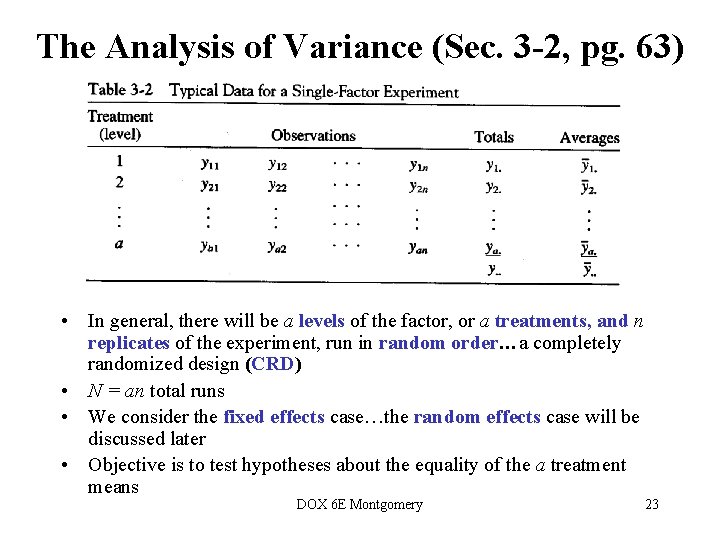
The Analysis of Variance (Sec. 3 -2, pg. 63) • In general, there will be a levels of the factor, or a treatments, and n replicates of the experiment, run in random order…a completely randomized design (CRD) • N = an total runs • We consider the fixed effects case…the random effects case will be discussed later • Objective is to test hypotheses about the equality of the a treatment means DOX 6 E Montgomery 23

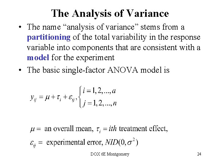
The Analysis of Variance • The name “analysis of variance” stems from a partitioning of the total variability in the response variable into components that are consistent with a model for the experiment • The basic single-factor ANOVA model is DOX 6 E Montgomery 24

Models for the Data There are several ways to write a model for the data: DOX 6 E Montgomery 25

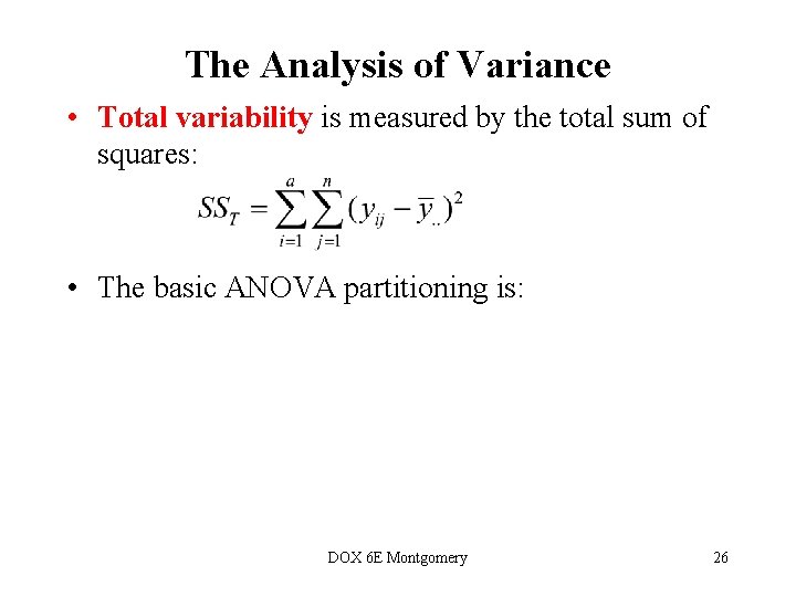
The Analysis of Variance • Total variability is measured by the total sum of squares: • The basic ANOVA partitioning is: DOX 6 E Montgomery 26

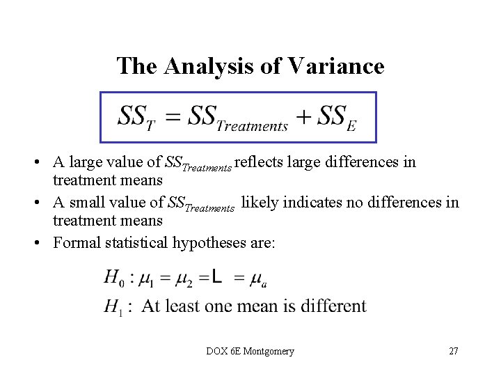
The Analysis of Variance • A large value of SSTreatments reflects large differences in treatment means • A small value of SSTreatments likely indicates no differences in treatment means • Formal statistical hypotheses are: DOX 6 E Montgomery 27

The Analysis of Variance • While sums of squares cannot be directly compared to test the hypothesis of equal means, mean squares can be compared. • A mean square is a sum of squares divided by its degrees of freedom: • If the treatment means are equal, the treatment and error mean squares will be (theoretically) equal. • If treatment means differ, the treatment mean square will be larger than the error mean square. DOX 6 E Montgomery 28

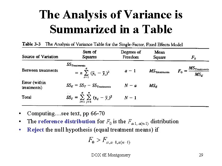
The Analysis of Variance is Summarized in a Table • Computing…see text, pp 66 -70 • The reference distribution for F 0 is the Fa-1, a(n-1) distribution • Reject the null hypothesis (equal treatment means) if DOX 6 E Montgomery 29

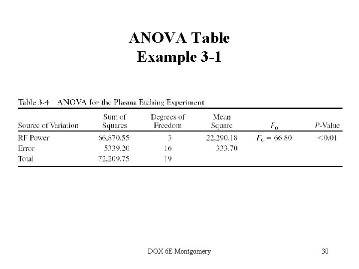
ANOVA Table Example 3 -1 DOX 6 E Montgomery 30

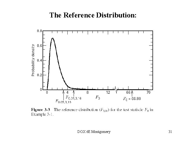
The Reference Distribution: DOX 6 E Montgomery 31

ANOVA calculations are usually done via computer • Text exhibits sample calculations from two very popular software packages, Design. Expert and Minitab • See page 99 for Design-Expert, page 100 for Minitab • Text discusses some of the summary statistics provided by these packages DOX 6 E Montgomery 32

Model Adequacy Checking in the ANOVA Text reference, Section 3 -4, pg. 75 • • • Checking assumptions is important Normality Constant variance Independence Have we fit the right model? Later we will talk about what to do if some of these assumptions are violated DOX 6 E Montgomery 33

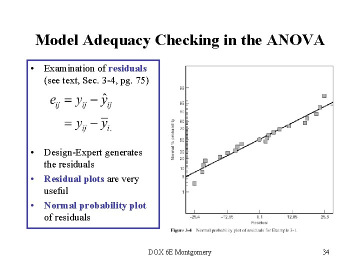
Model Adequacy Checking in the ANOVA • Examination of residuals (see text, Sec. 3 -4, pg. 75) • Design-Expert generates the residuals • Residual plots are very useful • Normal probability plot of residuals DOX 6 E Montgomery 34

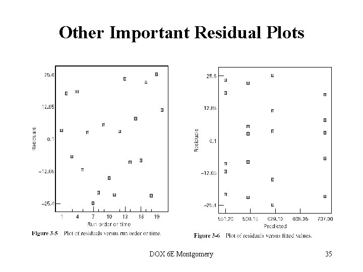
Other Important Residual Plots DOX 6 E Montgomery 35

Post-ANOVA Comparison of Means • The analysis of variance tests the hypothesis of equal treatment means • Assume that residual analysis is satisfactory • If that hypothesis is rejected, we don’t know which specific means are different • Determining which specific means differ following an ANOVA is called the multiple comparisons problem • There are lots of ways to do this…see text, Section 3 -5, pg. 87 • We will use pairwise t-tests on means…sometimes called Fisher’s Least Significant Difference (or Fisher’s LSD) Method DOX 6 E Montgomery 36

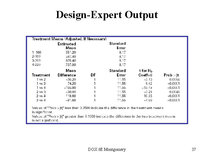
Design-Expert Output DOX 6 E Montgomery 37

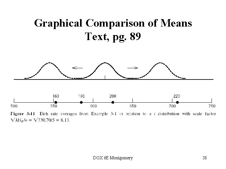
Graphical Comparison of Means Text, pg. 89 DOX 6 E Montgomery 38

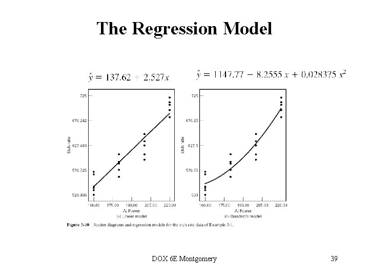
The Regression Model DOX 6 E Montgomery 39

Why Does the ANOVA Work? DOX 6 E Montgomery 40

Sample Size Determination Text, Section 3 -7, pg. 101 • FAQ in designed experiments • Answer depends on lots of things; including what type of experiment is being contemplated, how it will be conducted, resources, and desired sensitivity • Sensitivity refers to the difference in means that the experimenter wishes to detect • Generally, increasing the number of replications increases the sensitivity or it makes it easier to detect small differences in means DOX 6 E Montgomery 41

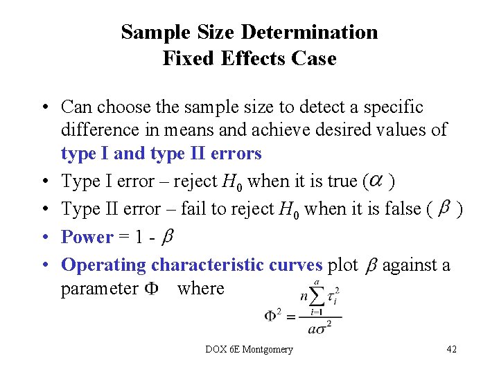
Sample Size Determination Fixed Effects Case • Can choose the sample size to detect a specific difference in means and achieve desired values of type I and type II errors • Type I error – reject H 0 when it is true ( ) • Type II error – fail to reject H 0 when it is false ( ) • Power = 1 • Operating characteristic curves plot against a parameter where DOX 6 E Montgomery 42

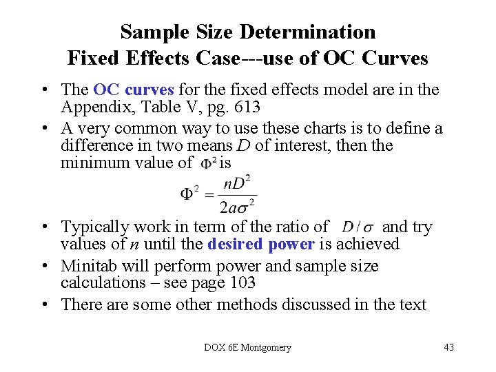
Sample Size Determination Fixed Effects Case---use of OC Curves • The OC curves for the fixed effects model are in the Appendix, Table V, pg. 613 • A very common way to use these charts is to define a difference in two means D of interest, then the minimum value of is • Typically work in term of the ratio of and try values of n until the desired power is achieved • Minitab will perform power and sample size calculations – see page 103 • There are some other methods discussed in the text DOX 6 E Montgomery 43

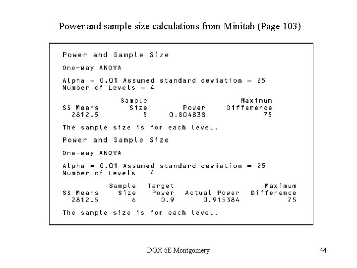
Power and sample size calculations from Minitab (Page 103) DOX 6 E Montgomery 44