Design of Digital Circuits Lecture 18 Branch Prediction

Design of Digital Circuits Lecture 18: Branch Prediction II Prof. Onur Mutlu ETH Zurich Spring 2019 2 May 2019
Required Readings n This week q q q Smith and Sohi, “The Microarchitecture of Superscalar Processors, ” Proceedings of the IEEE, 1995 H&H Chapters 7. 8 and 7. 9 Mc. Farling, “Combining Branch Predictors, ” DEC WRL Technical Report, 1993. 2
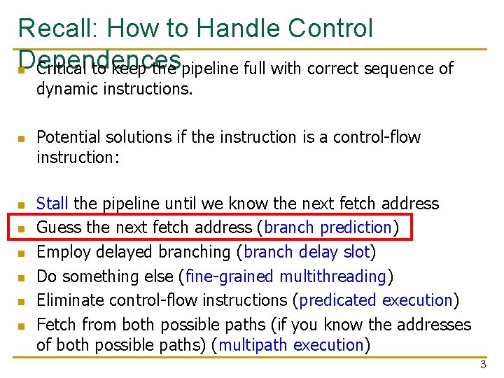
Recall: How to Handle Control Dependences n Critical to keep the pipeline full with correct sequence of dynamic instructions. n n n n Potential solutions if the instruction is a control-flow instruction: Stall the pipeline until we know the next fetch address Guess the next fetch address (branch prediction) Employ delayed branching (branch delay slot) Do something else (fine-grained multithreading) Eliminate control-flow instructions (predicated execution) Fetch from both possible paths (if you know the addresses of both possible paths) (multipath execution) 3
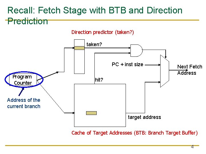
Recall: Fetch Stage with BTB and Direction Prediction Direction predictor (taken? ) taken? PC + inst size Program Counter Next Fetch Address hit? Address of the current branch target address Cache of Target Addresses (BTB: Branch Target Buffer) 4
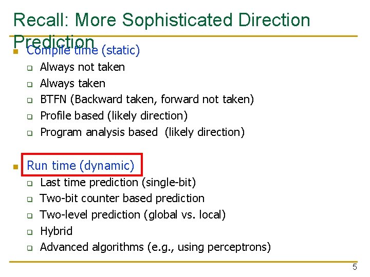
Recall: More Sophisticated Direction Prediction n Compile time (static) q q q n Always not taken Always taken BTFN (Backward taken, forward not taken) Profile based (likely direction) Program analysis based (likely direction) Run time (dynamic) q q q Last time prediction (single-bit) Two-bit counter based prediction Two-level prediction (global vs. local) Hybrid Advanced algorithms (e. g. , using perceptrons) 5
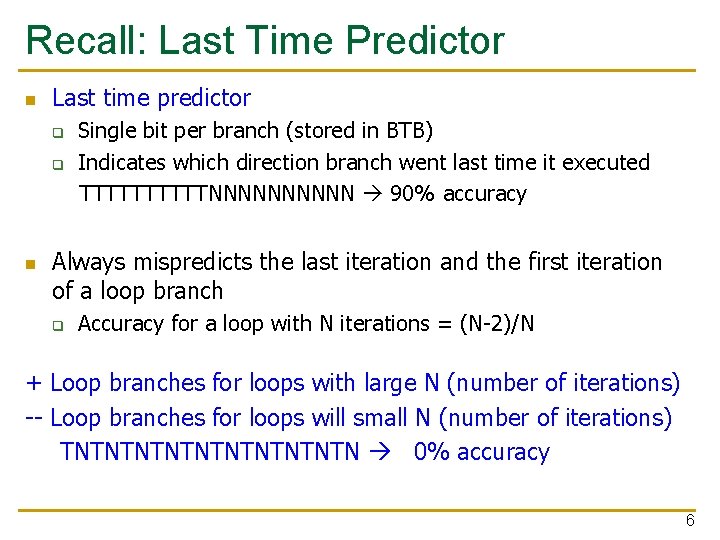
Recall: Last Time Predictor n Last time predictor q q n Single bit per branch (stored in BTB) Indicates which direction branch went last time it executed TTTTTNNNNN 90% accuracy Always mispredicts the last iteration and the first iteration of a loop branch q Accuracy for a loop with N iterations = (N-2)/N + Loop branches for loops with large N (number of iterations) -- Loop branches for loops will small N (number of iterations) TNTNTNTNTN 0% accuracy 6
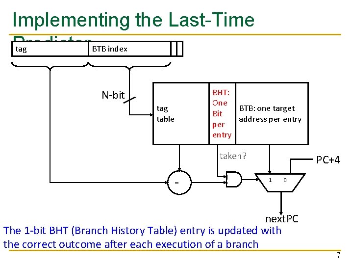
Implementing the Last-Time Predictor tag BTB index N-bit tag table BHT: One BTB: one target Bit address per entry taken? = PC+4 1 0 next. PC The 1 -bit BHT (Branch History Table) entry is updated with the correct outcome after each execution of a branch 7
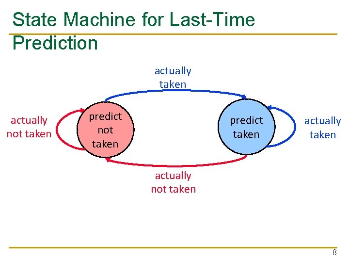
State Machine for Last-Time Prediction actually taken actually not taken predict taken actually not taken 8
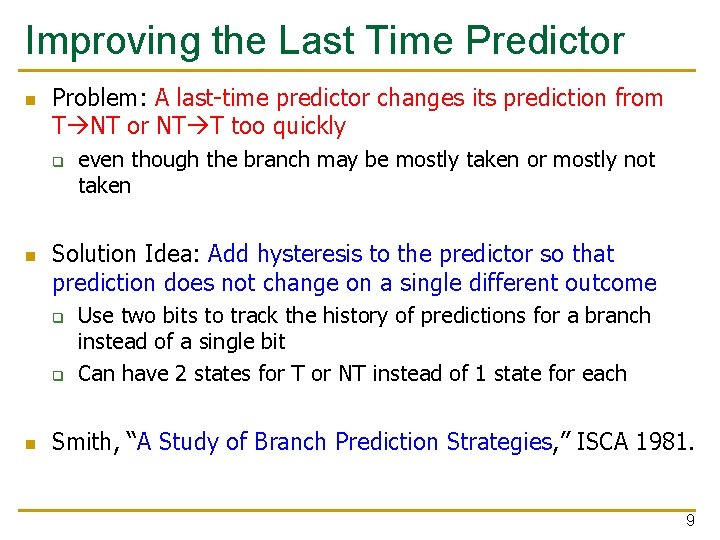
Improving the Last Time Predictor n Problem: A last-time predictor changes its prediction from T NT or NT T too quickly q n Solution Idea: Add hysteresis to the predictor so that prediction does not change on a single different outcome q q n even though the branch may be mostly taken or mostly not taken Use two bits to track the history of predictions for a branch instead of a single bit Can have 2 states for T or NT instead of 1 state for each Smith, “A Study of Branch Prediction Strategies, ” ISCA 1981. 9
Two-Bit Counter Based Prediction n Each branch associated with a two-bit counter One more bit provides hysteresis A strong prediction does not change with one single different outcome 10

State Machine for 2 -bit Saturating Counter using saturating arithmetic Counter Arithmetic with maximum and minimum values n q actually taken pred taken 11 actually !taken actually taken pred !taken 01 pred taken 10 actually !taken actually taken pred !taken 00 actually !taken 11
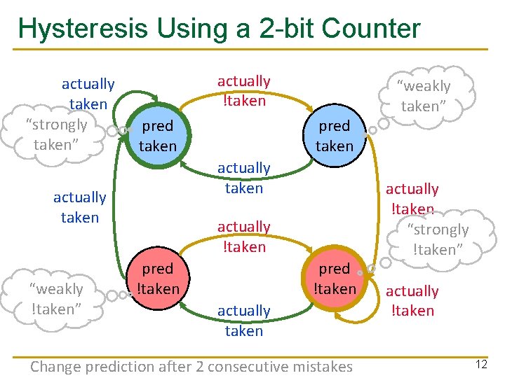
Hysteresis Using a 2 -bit Counter actually taken “strongly taken” actually !taken pred taken actually taken “weakly !taken” pred taken actually !taken pred !taken actually taken Change prediction after 2 consecutive mistakes “weakly taken” actually !taken “strongly !taken” actually !taken 12
Two-Bit Counter Based Prediction n n Each branch associated with a two-bit counter One more bit provides hysteresis A strong prediction does not change with one single different outcome Accuracy for a loop with N iterations = (N-1)/N TNTNTNTNTN 50% accuracy (assuming counter initialized to weakly taken) + Better prediction accuracy -- More hardware cost (but counter can be part of a BTB entry) 13
Is This Good Enough? n ~85 -90% accuracy for many programs with 2 -bit counter based prediction (also called bimodal prediction) n Is this good enough? n How big is the branch problem? 14
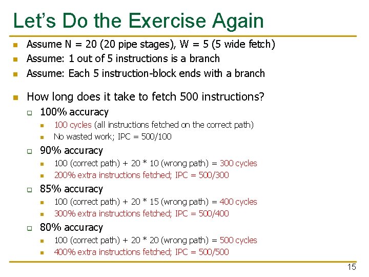
Let’s Do the Exercise Again n Assume N = 20 (20 pipe stages), W = 5 (5 wide fetch) Assume: 1 out of 5 instructions is a branch Assume: Each 5 instruction-block ends with a branch n How long does it take to fetch 500 instructions? n n q 100% accuracy n n q 90% accuracy n n q 100 (correct path) + 20 * 10 (wrong path) = 300 cycles 200% extra instructions fetched; IPC = 500/300 85% accuracy n n q 100 cycles (all instructions fetched on the correct path) No wasted work; IPC = 500/100 (correct path) + 20 * 15 (wrong path) = 400 cycles 300% extra instructions fetched; IPC = 500/400 80% accuracy n n 100 (correct path) + 20 * 20 (wrong path) = 500 cycles 400% extra instructions fetched; IPC = 500/500 15
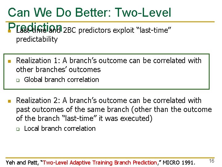
Can We Do Better: Two-Level Prediction n Last-time and 2 BC predictors exploit “last-time” predictability n Realization 1: A branch’s outcome can be correlated with other branches’ outcomes q n Global branch correlation Realization 2: A branch’s outcome can be correlated with past outcomes of the same branch (other than the outcome of the branch “last-time” it was executed) q Local branch correlation Yeh and Patt, “Two-Level Adaptive Training Branch Prediction, ” MICRO 1991. 16
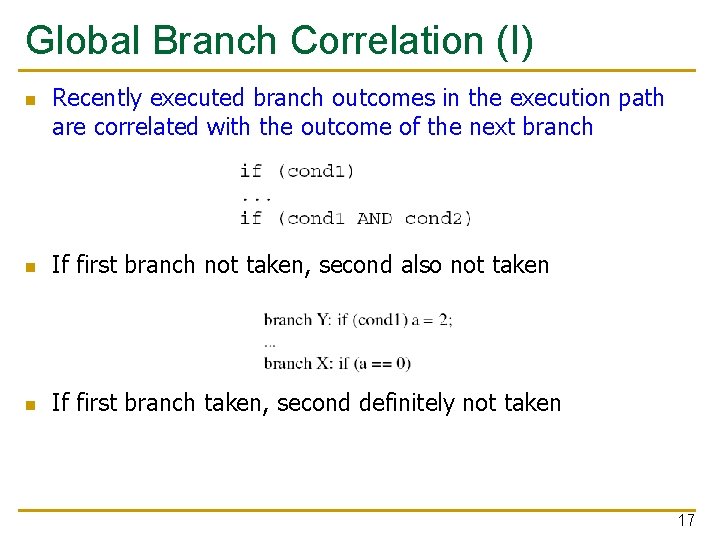
Global Branch Correlation (I) n Recently executed branch outcomes in the execution path are correlated with the outcome of the next branch n If first branch not taken, second also not taken n If first branch taken, second definitely not taken 17
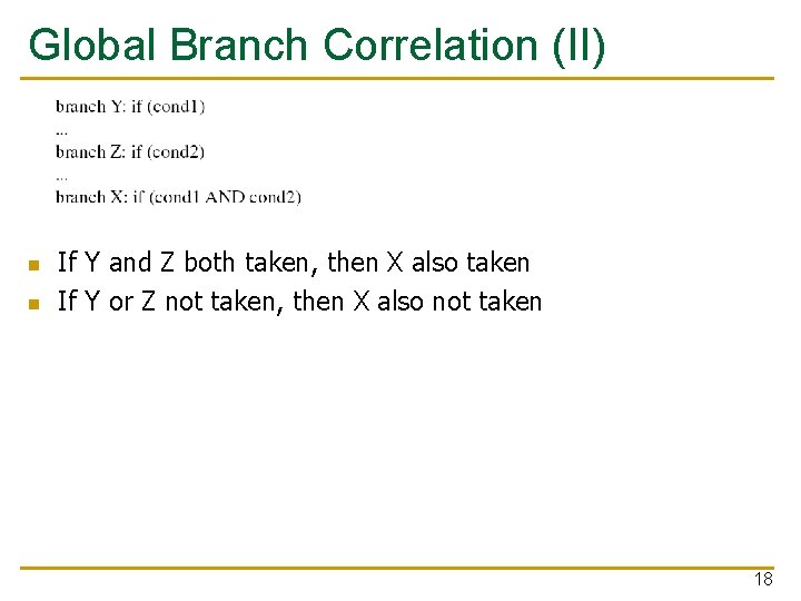
Global Branch Correlation (II) n n If Y and Z both taken, then X also taken If Y or Z not taken, then X also not taken 18
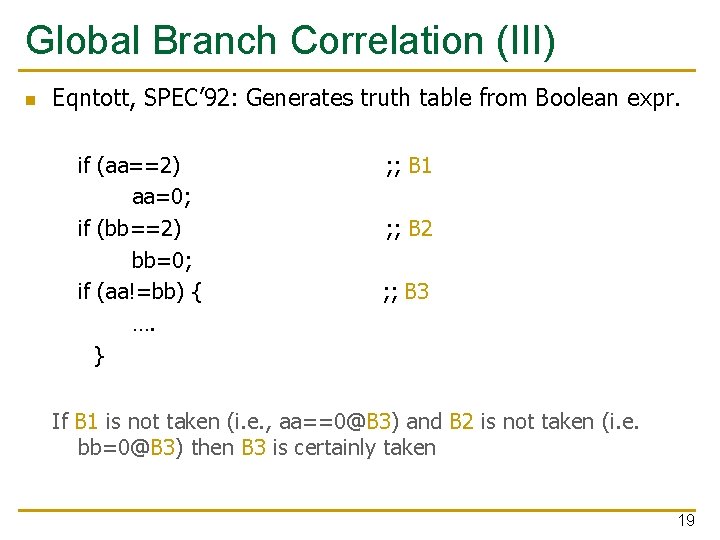
Global Branch Correlation (III) n Eqntott, SPEC’ 92: Generates truth table from Boolean expr. if (aa==2) aa=0; if (bb==2) bb=0; if (aa!=bb) { …. } ; ; B 1 ; ; B 2 ; ; B 3 If B 1 is not taken (i. e. , aa==0@B 3) and B 2 is not taken (i. e. bb=0@B 3) then B 3 is certainly taken 19
Capturing Global Branch Correlation n Idea: Associate branch outcomes with “global T/NT history” of all branches Make a prediction based on the outcome of the branch the last time the same global branch history was encountered Implementation: q q n n Keep track of the “global T/NT history” of all branches in a register Global History Register (GHR) Use GHR to index into a table that recorded the outcome that was seen for each GHR value in the recent past Pattern History Table (table of 2 -bit counters) Global history/branch predictor Uses two levels of history (GHR + history at that GHR) Yeh and Patt, “Two-Level Adaptive Training Branch Prediction, ” MICRO 1991. 20
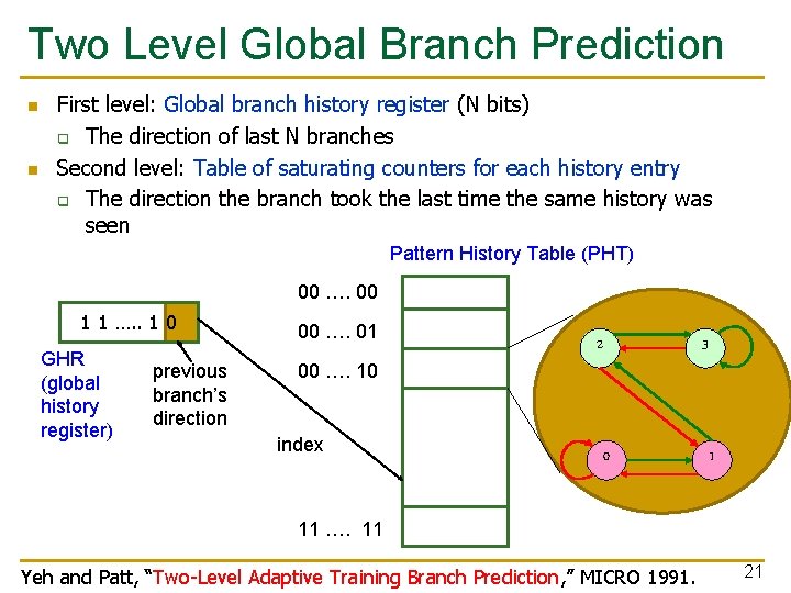
Two Level Global Branch Prediction n n First level: Global branch history register (N bits) q The direction of last N branches Second level: Table of saturating counters for each history entry q The direction the branch took the last time the same history was seen Pattern History Table (PHT) 00 …. 00 1 1 …. . 1 0 GHR (global history register) previous branch’s direction 00 …. 01 00 …. 10 index 2 3 0 1 11 …. 11 Yeh and Patt, “Two-Level Adaptive Training Branch Prediction, ” MICRO 1991. 21
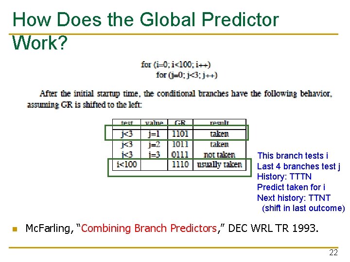
How Does the Global Predictor Work? This branch tests i Last 4 branches test j History: TTTN Predict taken for i Next history: TTNT (shift in last outcome) n Mc. Farling, “Combining Branch Predictors, ” DEC WRL TR 1993. 22
Intel Pentium Pro Branch Predictor n n n Two level global branch predictor 4 -bit global history register Multiple pattern history tables (of 2 bit counters) q n Which pattern history table to use is determined by lower order bits of the branch address First widely commercially successful out-of-order execution machine 23
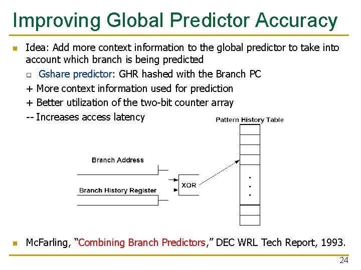
Improving Global Predictor Accuracy n n Idea: Add more context information to the global predictor to take into account which branch is being predicted q Gshare predictor: GHR hashed with the Branch PC + More context information used for prediction + Better utilization of the two-bit counter array -- Increases access latency Mc. Farling, “Combining Branch Predictors, ” DEC WRL Tech Report, 1993. 24
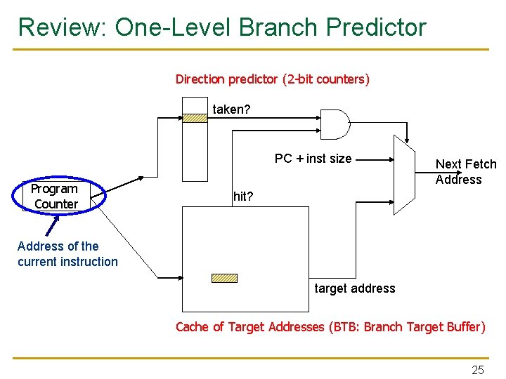
Review: One-Level Branch Predictor Direction predictor (2 -bit counters) taken? PC + inst size Program Counter Next Fetch Address hit? Address of the current instruction target address Cache of Target Addresses (BTB: Branch Target Buffer) 25
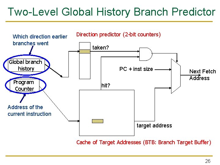
Two-Level Global History Branch Predictor Which direction earlier branches went Direction predictor (2 -bit counters) taken? Global branch history Program Counter PC + inst size Next Fetch Address hit? Address of the current instruction target address Cache of Target Addresses (BTB: Branch Target Buffer) 26
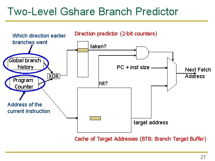
Two-Level Gshare Branch Predictor Which direction earlier branches went Direction predictor (2 -bit counters) taken? Global branch history Program Counter PC + inst size XOR Next Fetch Address hit? Address of the current instruction target address Cache of Target Addresses (BTB: Branch Target Buffer) 27
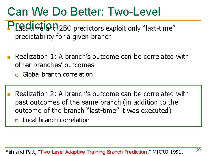
Can We Do Better: Two-Level Prediction n Last-time and 2 BC predictors exploit only “last-time” predictability for a given branch n Realization 1: A branch’s outcome can be correlated with other branches’ outcomes q n Global branch correlation Realization 2: A branch’s outcome can be correlated with past outcomes of the same branch (in addition to the outcome of the branch “last-time” it was executed) q Local branch correlation Yeh and Patt, “Two-Level Adaptive Training Branch Prediction, ” MICRO 1991. 28
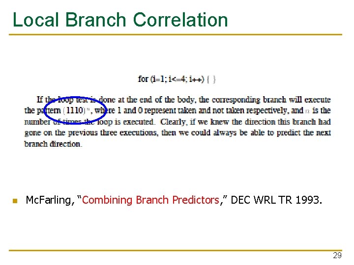
Local Branch Correlation n Mc. Farling, “Combining Branch Predictors, ” DEC WRL TR 1993. 29
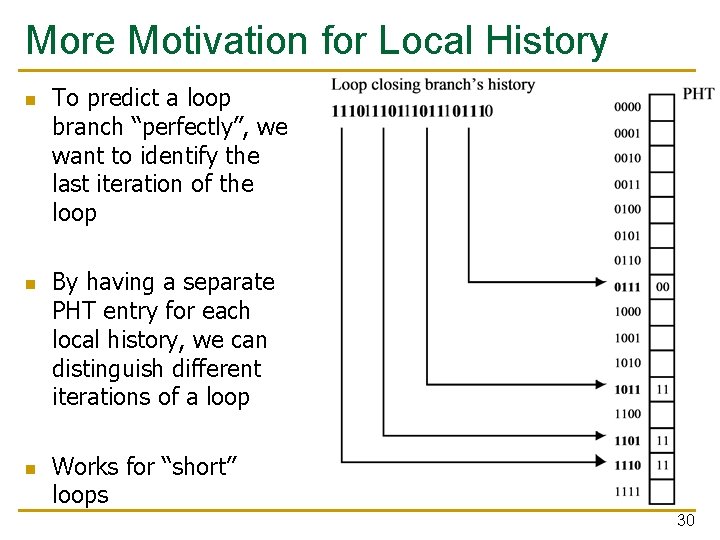
More Motivation for Local History n n n To predict a loop branch “perfectly”, we want to identify the last iteration of the loop By having a separate PHT entry for each local history, we can distinguish different iterations of a loop Works for “short” loops 30
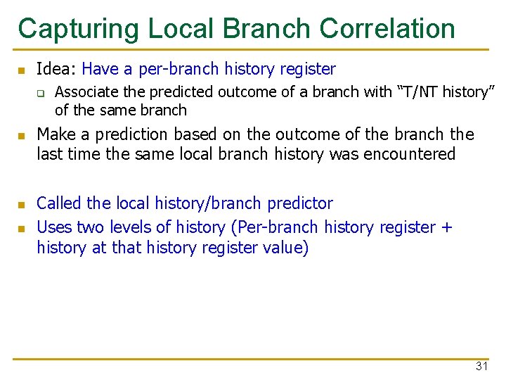
Capturing Local Branch Correlation n Idea: Have a per-branch history register q n n n Associate the predicted outcome of a branch with “T/NT history” of the same branch Make a prediction based on the outcome of the branch the last time the same local branch history was encountered Called the local history/branch predictor Uses two levels of history (Per-branch history register + history at that history register value) 31
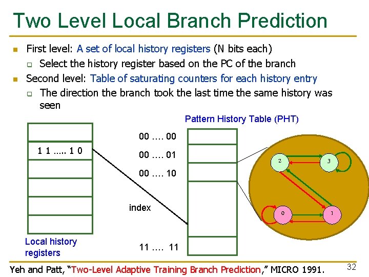
Two Level Local Branch Prediction n n First level: A set of local history registers (N bits each) q Select the history register based on the PC of the branch Second level: Table of saturating counters for each history entry q The direction the branch took the last time the same history was seen Pattern History Table (PHT) 00 …. 00 1 1 …. . 1 0 00 …. 01 00 …. 10 index Local history registers 2 3 0 1 11 …. 11 Yeh and Patt, “Two-Level Adaptive Training Branch Prediction, ” MICRO 1991. 32
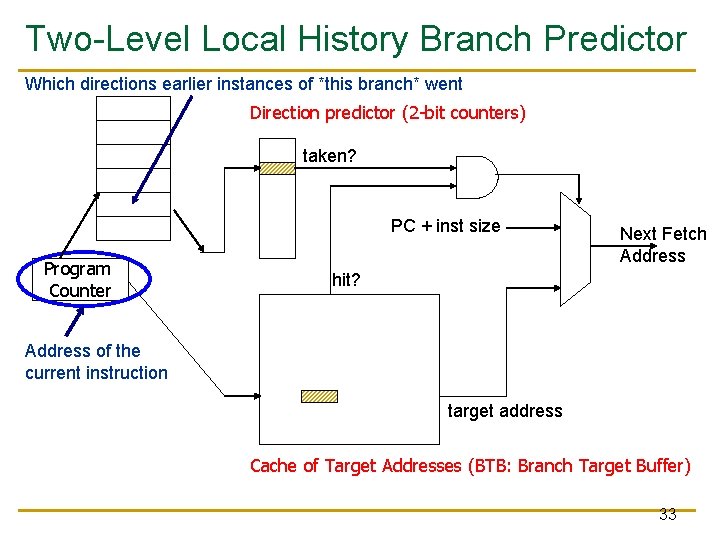
Two-Level Local History Branch Predictor Which directions earlier instances of *this branch* went Direction predictor (2 -bit counters) taken? PC + inst size Program Counter Next Fetch Address hit? Address of the current instruction target address Cache of Target Addresses (BTB: Branch Target Buffer) 33
Can We Do Even Better? n n n Predictability of branches varies Some branches are more predictable using local history Some branches are more predictable using global For others, a simple two-bit counter is enough Yet for others, a single bit is enough Observation: There is heterogeneity in predictability behavior of branches q n No one-size fits all branch prediction algorithm for all branches Idea: Exploit that heterogeneity by designing heterogeneous (hybrid) branch predictors 34
Hybrid Branch Predictors n Idea: Use more than one type of predictor (i. e. , multiple algorithms) and select the “best” prediction q n E. g. , hybrid of 2 -bit counters and global predictor Advantages: + Better accuracy: different predictors are better for different branches + Reduced warmup time (faster-warmup predictor used until the slower -warmup predictor warms up) n Disadvantages: -- Need “meta-predictor” or “selector” to decide which predictor to use -- Longer access latency q Mc. Farling, “Combining Branch Predictors, ” DEC WRL Tech Report, 1993. 35
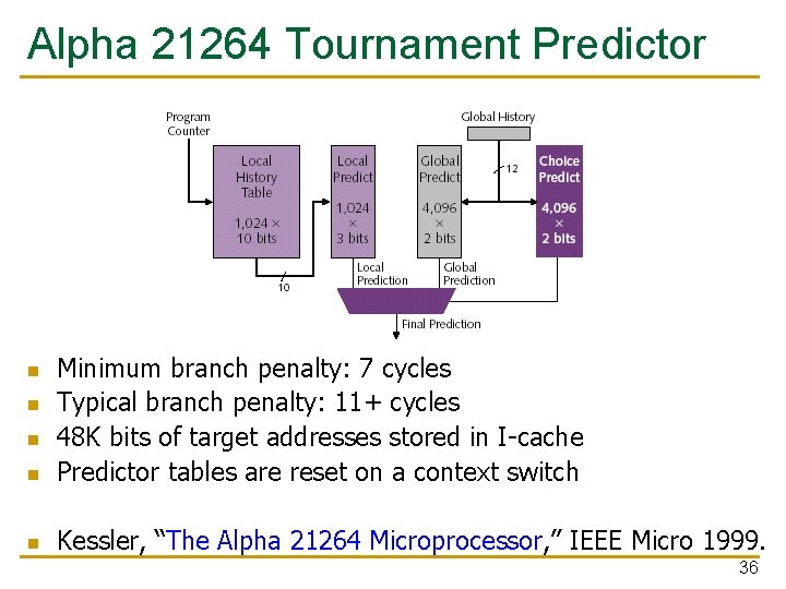
Alpha 21264 Tournament Predictor n Minimum branch penalty: 7 cycles Typical branch penalty: 11+ cycles 48 K bits of target addresses stored in I-cache Predictor tables are reset on a context switch n Kessler, “The Alpha 21264 Microprocessor, ” IEEE Micro 1999. n n n 36
Are We Done w/ Branch Prediction? n Hybrid branch predictors work well q n E. g. , 90 -97% prediction accuracy on average Some “difficult” workloads still suffer, though! q q q E. g. , gcc Max IPC with tournament prediction: 9 Max IPC with perfect prediction: 35 37
Some Other Branch Predictor Types n Loop branch detector and predictor q q q n Perceptron branch predictor q Learns the direction correlations between individual branches q q n Loop iteration count detector/predictor Works well for loops with small number of iterations, where iteration count is predictable Used in Intel Pentium M Assigns weights to correlations Jimenez and Lin, “Dynamic Branch Prediction with Perceptrons, ” HPCA 2001. Hybrid history length based predictor q q Uses different tables with different history lengths Seznec, “Analysis of the O-Geometric History Length branch predictor, ” ISCA 2005. 38
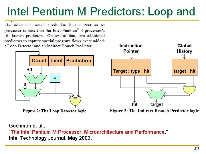
Intel Pentium M Predictors: Loop and Jump Gochman et al. , “The Intel Pentium M Processor: Microarchitecture and Performance, ” Intel Technology Journal, May 2003. 39
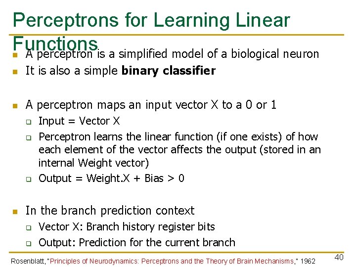
Perceptrons for Learning Linear Functions n A perceptron is a simplified model of a biological neuron n It is also a simple binary classifier n A perceptron maps an input vector X to a 0 or 1 q q q n Input = Vector X Perceptron learns the linear function (if one exists) of how each element of the vector affects the output (stored in an internal Weight vector) Output = Weight. X + Bias > 0 In the branch prediction context q q Vector X: Branch history register bits Output: Prediction for the current branch Rosenblatt, “Principles of Neurodynamics: Perceptrons and the Theory of Brain Mechanisms, ” 1962 40
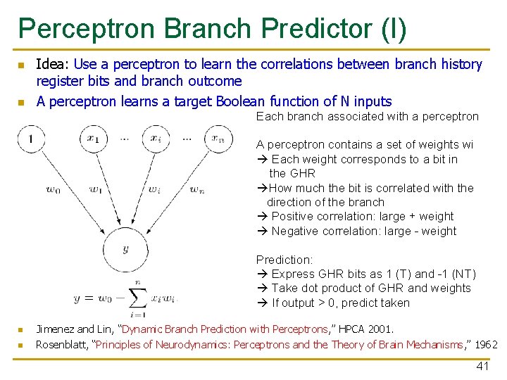
Perceptron Branch Predictor (I) n n Idea: Use a perceptron to learn the correlations between branch history register bits and branch outcome A perceptron learns a target Boolean function of N inputs Each branch associated with a perceptron A perceptron contains a set of weights wi Each weight corresponds to a bit in the GHR How much the bit is correlated with the direction of the branch Positive correlation: large + weight Negative correlation: large - weight Prediction: Express GHR bits as 1 (T) and -1 (NT) Take dot product of GHR and weights If output > 0, predict taken n n Jimenez and Lin, “Dynamic Branch Prediction with Perceptrons, ” HPCA 2001. Rosenblatt, “Principles of Neurodynamics: Perceptrons and the Theory of Brain Mechanisms, ” 1962 41
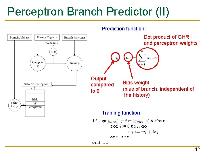
Perceptron Branch Predictor (II) Prediction function: Dot product of GHR and perceptron weights Output compared to 0 Bias weight (bias of branch, independent of the history) Training function: 42
Perceptron Branch Predictor (III) n Advantages + More sophisticated learning mechanism better accuracy n Disadvantages -- Hard to implement (adder tree to compute perceptron output) -- Can learn only linearly-separable functions e. g. , cannot learn XOR type of correlation between 2 history bits and branch outcome A successful example of use of machine learning in processor design 43
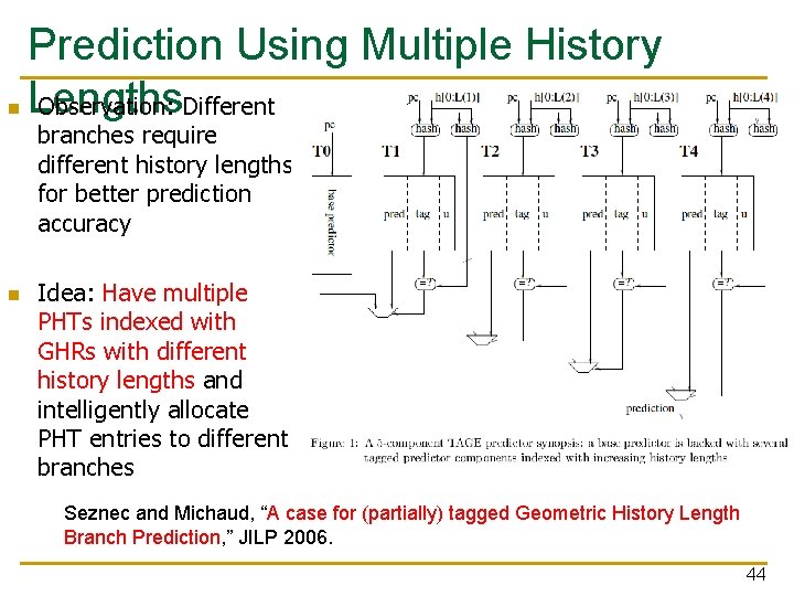
n Prediction Using Multiple History Lengths Observation: Different branches require different history lengths for better prediction accuracy n Idea: Have multiple PHTs indexed with GHRs with different history lengths and intelligently allocate PHT entries to different branches Seznec and Michaud, “A case for (partially) tagged Geometric History Length Branch Prediction, ” JILP 2006. 44
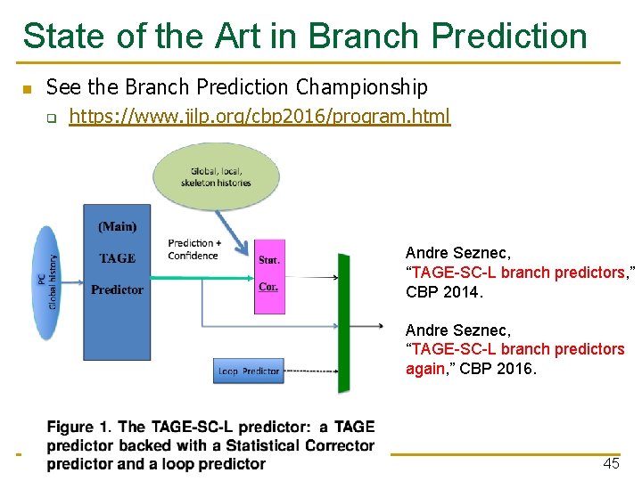
State of the Art in Branch Prediction n See the Branch Prediction Championship q https: //www. jilp. org/cbp 2016/program. html Andre Seznec, “TAGE-SC-L branch predictors, ” CBP 2014. Andre Seznec, “TAGE-SC-L branch predictors again, ” CBP 2016. 45
Branch Confidence Estimation n Idea: Estimate if the prediction is likely to be correct q n i. e. , estimate how “confident” you are in the prediction Why? q Could be very useful in deciding how to speculate: n n n What predictor/PHT to choose/use Whether to keep fetching on this path Whether to switch to some other way of handling the branch, e. g. dual-path execution (eager execution) or dynamic predication … Jacobsen et al. , “Assigning Confidence to Conditional Branch Predictions, ” MICRO 1996. 46

Other Ways of Handling Branches 47
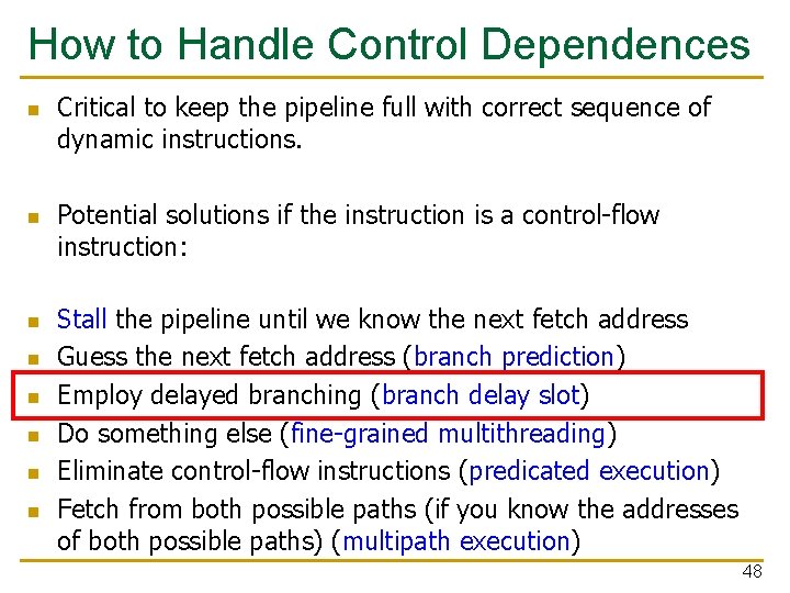
How to Handle Control Dependences n n n n Critical to keep the pipeline full with correct sequence of dynamic instructions. Potential solutions if the instruction is a control-flow instruction: Stall the pipeline until we know the next fetch address Guess the next fetch address (branch prediction) Employ delayed branching (branch delay slot) Do something else (fine-grained multithreading) Eliminate control-flow instructions (predicated execution) Fetch from both possible paths (if you know the addresses of both possible paths) (multipath execution) 48
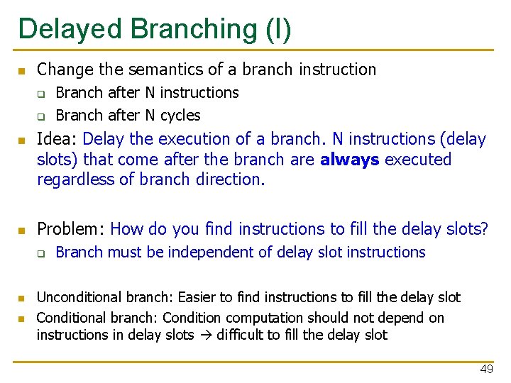
Delayed Branching (I) n Change the semantics of a branch instruction q q n n Idea: Delay the execution of a branch. N instructions (delay slots) that come after the branch are always executed regardless of branch direction. Problem: How do you find instructions to fill the delay slots? q n n Branch after N instructions Branch after N cycles Branch must be independent of delay slot instructions Unconditional branch: Easier to find instructions to fill the delay slot Conditional branch: Condition computation should not depend on instructions in delay slots difficult to fill the delay slot 49
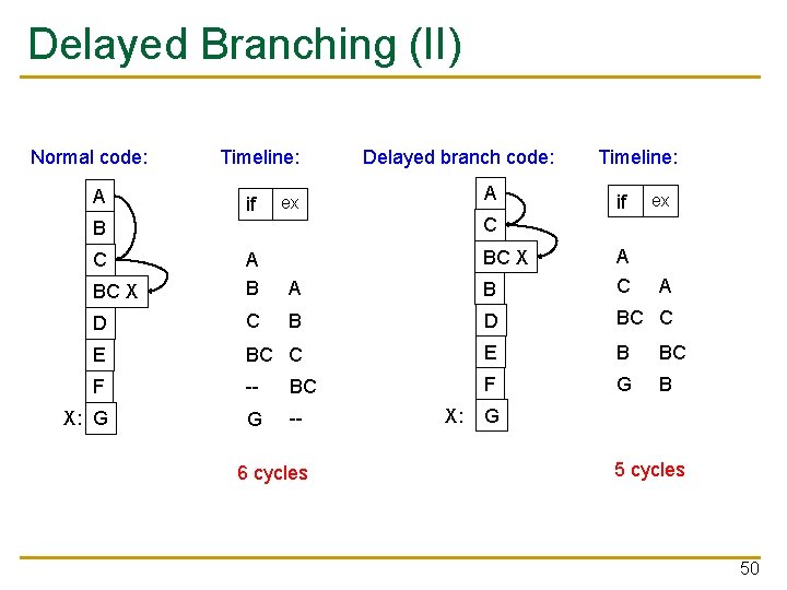
Delayed Branching (II) Normal code: A Timeline: if Delayed branch code: A ex Timeline: if ex A C B BC X A B A C D C B D BC C E B BC F -- BC F G B X: G G -- C BC X 6 cycles X: G 5 cycles 50
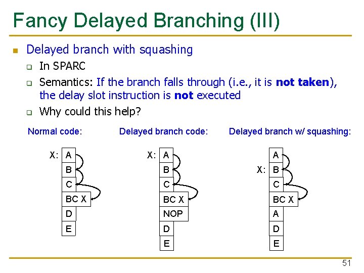
Fancy Delayed Branching (III) n Delayed branch with squashing q q q In SPARC Semantics: If the branch falls through (i. e. , it is not taken), the delay slot instruction is not executed Why could this help? Normal code: Delayed branch w/ squashing: X: A A B B X: B C C C BC X D NOP A E D D E E 51
Delayed Branching (IV) n Advantages: + Keeps the pipeline full with useful instructions in a simple way assuming 1. Number of delay slots == number of instructions to keep the pipeline full before the branch resolves 2. All delay slots can be filled with useful instructions n Disadvantages: -- Not easy to fill the delay slots (even with a 2 -stage pipeline) 1. Number of delay slots increases with pipeline depth, superscalar execution width 2. Number of delay slots should be variable with variable latency operations. Why? -- Ties ISA semantics to hardware implementation -- SPARC, MIPS, HP-PA: 1 delay slot -- What if pipeline implementation changes with the next design? 52

Design of Digital Circuits Lecture 18: Branch Prediction II Prof. Onur Mutlu ETH Zurich Spring 2019 2 May 2019

We did not cover the following slides. They are for your benefit. 54
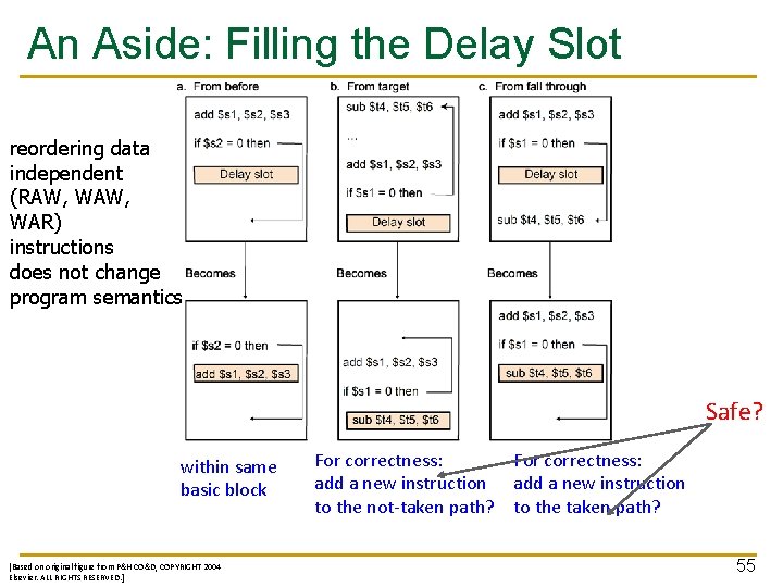
An Aside: Filling the Delay Slot reordering data independent (RAW, WAR) instructions does not change program semantics Safe? within same basic block [Based on original figure from P&H CO&D, COPYRIGHT 2004 Elsevier. ALL RIGHTS RESERVED. ] For correctness: add a new instruction to the not-taken path? to the taken path? 55
How to Handle Control Dependences n n n n Critical to keep the pipeline full with correct sequence of dynamic instructions. Potential solutions if the instruction is a control-flow instruction: Stall the pipeline until we know the next fetch address Guess the next fetch address (branch prediction) Employ delayed branching (branch delay slot) Do something else (fine-grained multithreading) Eliminate control-flow instructions (predicated execution) Fetch from both possible paths (if you know the addresses of both possible paths) (multipath execution) 56
Predicate Combining (not Predicated Execution) n Complex predicates are converted into multiple branches q if ((a == b) && (c < d) && (a > 5000)) { … } n n n 3 conditional branches Problem: This increases the number of control dependencies Idea: Combine predicate operations to feed a single branch instruction instead of having one branch for each q q Predicates stored and operated on using condition registers A single branch checks the value of the combined predicate + Fewer branches in code fewer mipredictions/stalls -- Possibly unnecessary work n -- If the first predicate is false, no need to compute other predicates Condition registers exist in IBM RS 6000 and the POWER architecture 57
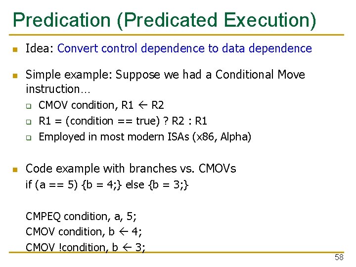
Predication (Predicated Execution) n n Idea: Convert control dependence to data dependence Simple example: Suppose we had a Conditional Move instruction… q q q n CMOV condition, R 1 R 2 R 1 = (condition == true) ? R 2 : R 1 Employed in most modern ISAs (x 86, Alpha) Code example with branches vs. CMOVs if (a == 5) {b = 4; } else {b = 3; } CMPEQ condition, a, 5; CMOV condition, b 4; CMOV !condition, b 3; 58
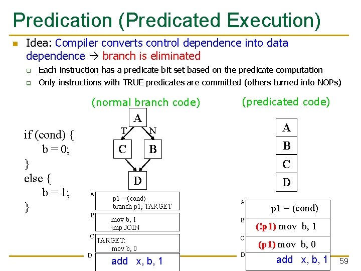
Predication (Predicated Execution) n Idea: Compiler converts control dependence into data dependence branch is eliminated q q Each instruction has a predicate bit set based on the predicate computation Only instructions with TRUE predicates are committed (others turned into NOPs) (normal branch code) (predicated code) A if (cond) { b = 0; } else { b = 1; } T N C B A B C D p 1 = (cond) branch p 1, TARGET mov b, 1 jmp JOIN TARGET: mov b, 0 add x, b, 1 D A B C D p 1 = (cond) (!p 1) mov b, 1 (p 1) mov b, 0 add x, b, 1 59
Predicated Execution References n n Allen et al. , “Conversion of control dependence to data dependence, ” POPL 1983. Kim et al. , “Wish Branches: Combining Conditional Branching and Predication for Adaptive Predicated Execution, ” MICRO 2005. 60
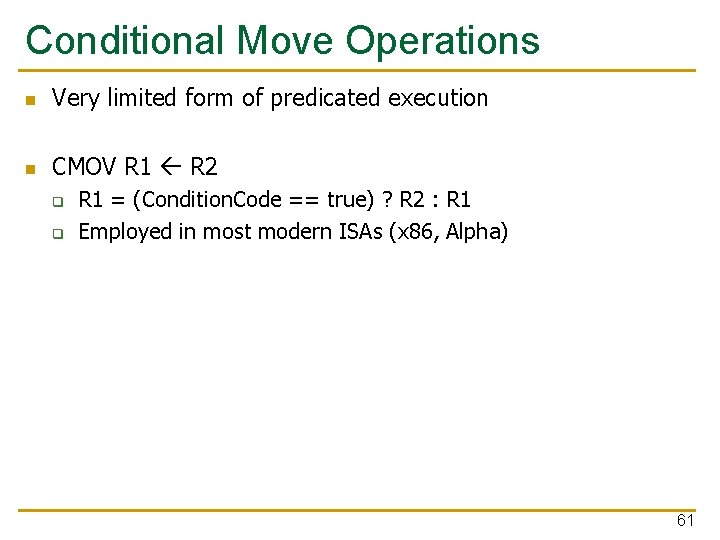
Conditional Move Operations n Very limited form of predicated execution n CMOV R 1 R 2 q q R 1 = (Condition. Code == true) ? R 2 : R 1 Employed in most modern ISAs (x 86, Alpha) 61
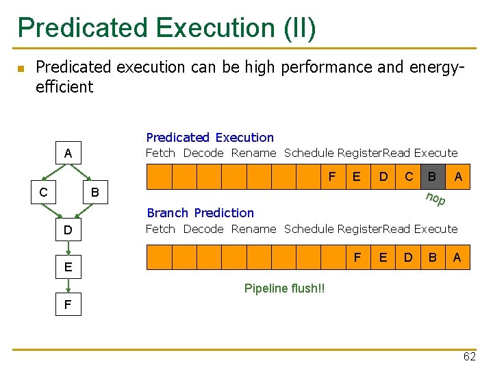
Predicated Execution (II) n Predicated execution can be high performance and energyefficient Predicated Execution Fetch Decode Rename Schedule Register. Read Execute A F E A D B C C E F D C A B F E D C B A A C D B E F C B A D E F A B D C E F A D F C E B F D C A E B C D A B E B C A D C A B B Branch Prediction D B A A nop Fetch Decode Rename Schedule Register. Read Execute F E E D B A Pipeline flush!! F 62
Predicated Execution n n Eliminates branches enables straight line code (i. e. , larger basic blocks in code) Advantages q q q Eliminates hard-to-predict branches Always-not-taken prediction works better (no branches) Compiler has more freedom to optimize code (no branches) n n n control flow does not hinder inst. reordering optimizations code optimizations hindered only by data dependencies Disadvantages q q q Useless work: some instructions fetched/executed but discarded (especially bad for easy-to-predict branches) Requires additional ISA (and hardware) support Can we eliminate all branches this way? 63
Predicated Execution vs. Branch + Eliminates mispredictions for hard-to-predict branches Prediction + No need for branch prediction for some branches + Good if misprediction cost > useless work due to predication -- Causes useless work for branches that are easy to predict -- Reduces performance if misprediction cost < useless work -- Adaptivity: Static predication is not adaptive to run-time branch behavior. Branch behavior changes based on input set, program phase, control-flow path. 64
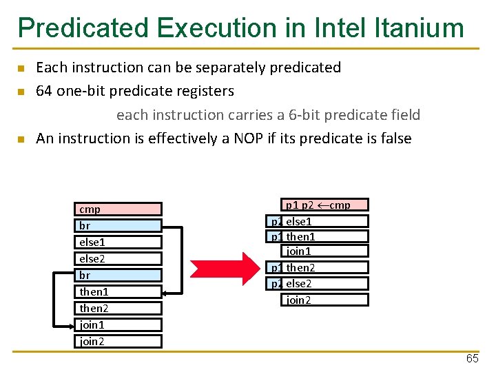
Predicated Execution in Intel Itanium n n n Each instruction can be separately predicated 64 one-bit predicate registers each instruction carries a 6 -bit predicate field An instruction is effectively a NOP if its predicate is false cmp br else 1 else 2 br then 1 then 2 join 1 join 2 p 1 p 2 cmp p 2 else 1 p 1 then 1 join 1 p 1 then 2 p 2 else 2 join 2 65
Conditional Execution in the ARM ISA n Almost all ARM instructions could include an optional condition code. q n Prior to ARM v 8 An instruction with a condition code is executed only if the condition code flags in the CPSR meet the specified condition. 66
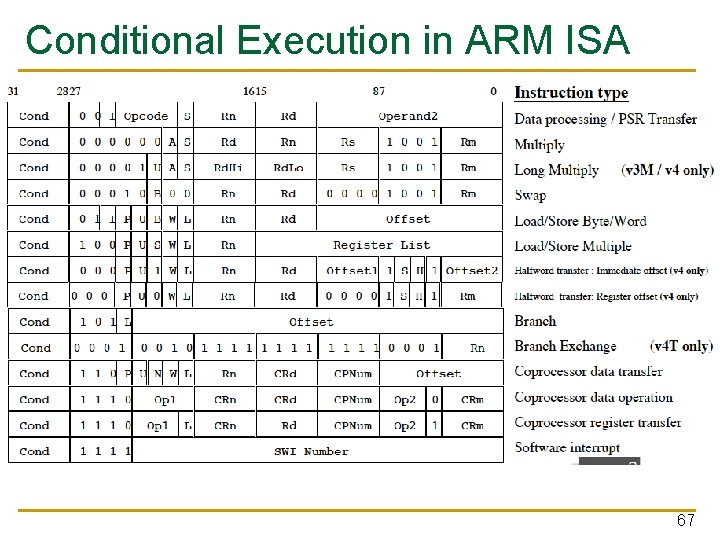
Conditional Execution in ARM ISA 67
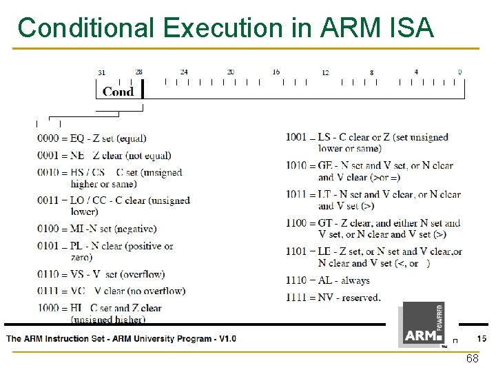
Conditional Execution in ARM ISA 68
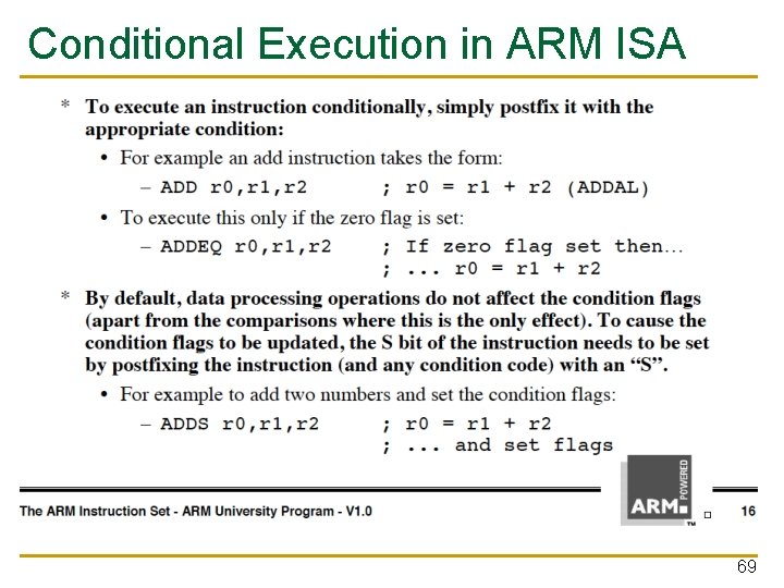
Conditional Execution in ARM ISA 69
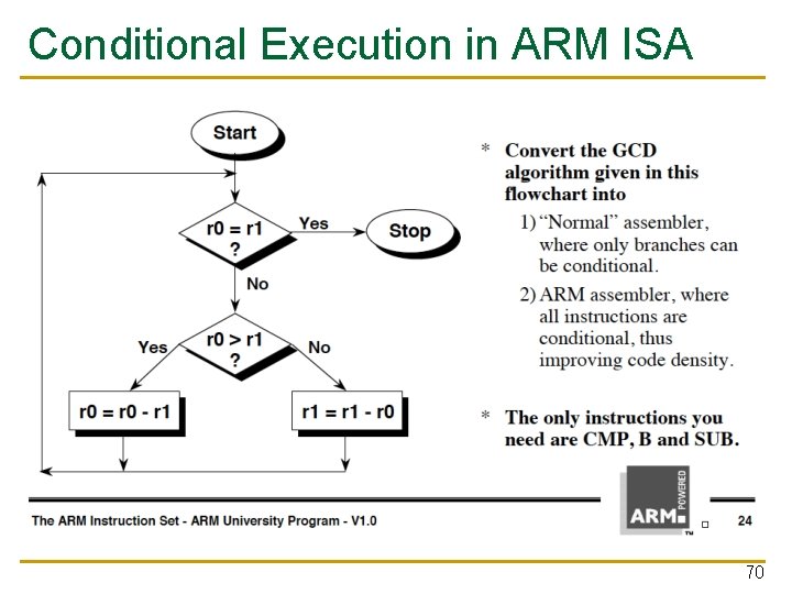
Conditional Execution in ARM ISA 70
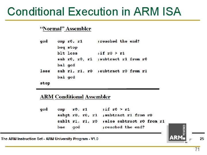
Conditional Execution in ARM ISA 71
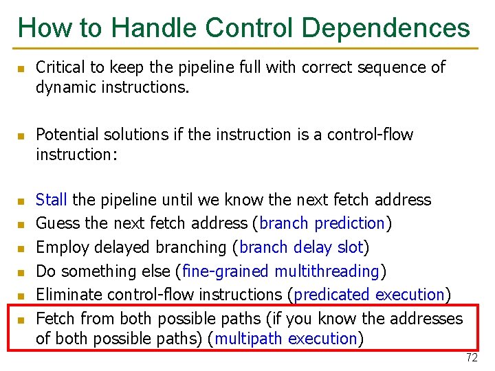
How to Handle Control Dependences n n n n Critical to keep the pipeline full with correct sequence of dynamic instructions. Potential solutions if the instruction is a control-flow instruction: Stall the pipeline until we know the next fetch address Guess the next fetch address (branch prediction) Employ delayed branching (branch delay slot) Do something else (fine-grained multithreading) Eliminate control-flow instructions (predicated execution) Fetch from both possible paths (if you know the addresses of both possible paths) (multipath execution) 72
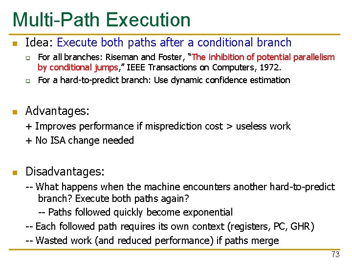
Multi-Path Execution n Idea: Execute both paths after a conditional branch q q n For all branches: Riseman and Foster, “The inhibition of potential parallelism by conditional jumps, ” IEEE Transactions on Computers, 1972. For a hard-to-predict branch: Use dynamic confidence estimation Advantages: + Improves performance if misprediction cost > useless work + No ISA change needed n Disadvantages: -- What happens when the machine encounters another hard-to-predict branch? Execute both paths again? -- Paths followed quickly become exponential -- Each followed path requires its own context (registers, PC, GHR) -- Wasted work (and reduced performance) if paths merge 73
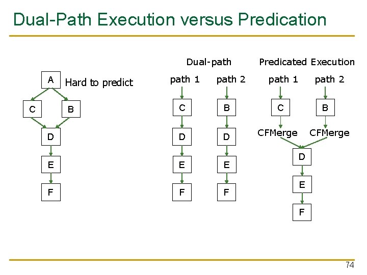
Dual-Path Execution versus Predication Dual-path A C Hard to predict B D E F path 1 path 2 C B D D E F Predicated Execution path 1 path 2 C B CFMerge D E F 74
Handling Other Types of Branches 75
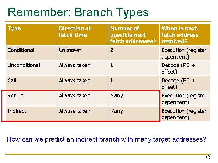
Remember: Branch Types Type Direction at fetch time Number of When is next possible next fetch addresses? resolved? Conditional Unknown 2 Execution (register dependent) Unconditional Always taken 1 Decode (PC + offset) Call Always taken 1 Decode (PC + offset) Return Always taken Many Execution (register dependent) Indirect Always taken Many Execution (register dependent) How can we predict an indirect branch with many target addresses? 76
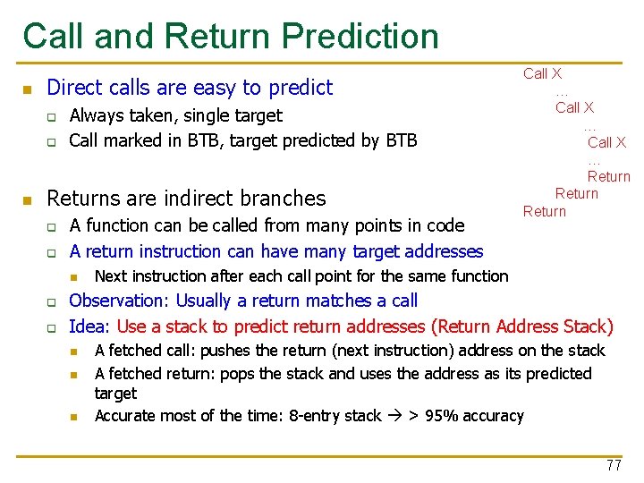
Call and Return Prediction n Direct calls are easy to predict q q n Always taken, single target Call marked in BTB, target predicted by BTB Returns are indirect branches q q A function can be called from many points in code A return instruction can have many target addresses n q q Call X … Return Next instruction after each call point for the same function Observation: Usually a return matches a call Idea: Use a stack to predict return addresses (Return Address Stack) n n n A fetched call: pushes the return (next instruction) address on the stack A fetched return: pops the stack and uses the address as its predicted target Accurate most of the time: 8 -entry stack > 95% accuracy 77
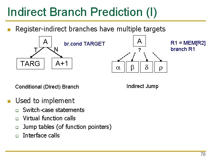
Indirect Branch Prediction (I) n Register-indirect branches have multiple targets A T TARG N A+1 Conditional (Direct) Branch n A br. cond TARGET R 1 = MEM[R 2] branch R 1 ? a b d r Indirect Jump Used to implement q q Switch-case statements Virtual function calls Jump tables (of function pointers) Interface calls 78
Indirect Branch Prediction (II) n n No direction prediction needed Idea 1: Predict the last resolved target as the next fetch address + Simple: Use the BTB to store the target address -- Inaccurate: 50% accuracy (empirical). Many indirect branches switch between different targets n Idea 2: Use history based target prediction E. g. , Index the BTB with GHR XORed with Indirect Branch PC q Chang et al. , “Target Prediction for Indirect Jumps, ” ISCA 1997. + More accurate -- An indirect branch maps to (too) many entries in BTB -- Conflict misses with other branches (direct or indirect) -- Inefficient use of space if branch has few target addresses q 79
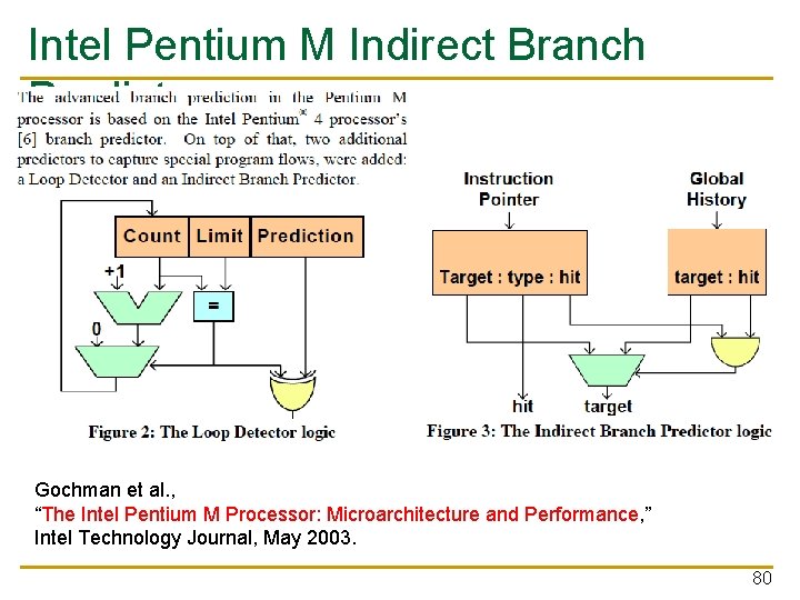
Intel Pentium M Indirect Branch Predictor Gochman et al. , “The Intel Pentium M Processor: Microarchitecture and Performance, ” Intel Technology Journal, May 2003. 80
Issues in Branch Prediction (I) n Need to identify a branch before it is fetched n How do we do this? q q q n BTB hit indicates that the fetched instruction is a branch BTB entry contains the “type” of the branch Pre-decoded “branch type” information stored in the instruction cache identifies type of branch What if no BTB? q q Bubble in the pipeline until target address is computed E. g. , IBM POWER 4 81
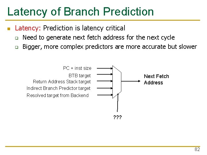
Latency of Branch Prediction n Latency: Prediction is latency critical q q Need to generate next fetch address for the next cycle Bigger, more complex predictors are more accurate but slower PC + inst size BTB target Return Address Stack target Indirect Branch Predictor target Next Fetch Address Resolved target from Backend ? ? ? 82
- Slides: 82