DESIGN METHOD OF FIR FILTER WINDOWING TECHNIQUES The

DESIGN METHOD OF FIR FILTER – WINDOWING TECHNIQUES

The window method A suitable window function w[n] is selected, required word length is calculated. Then it is multiplied with the impulse response of a (ideal) LPF. Thus hw [n] = h[n] w[n] Or, hw [n] = H[F] W[F].

The window method…. n n The spectrum of ideal low pass filter have a jump discontinuity at F = Fc. But the windowed spectrum shows over-shoot, ripple and a finite transition width but no abrupt jump.

Window method contd… It’s normalized signal magnitude at F = Fc is 0. 5. It corresponds to attenuation of -6 d. B. The ripple in pass band over-shoot is attributed to Gibb’s phenomena; 9% minimum. The side-lobs produces the ripple in pass band stop band. The ripples in pass band stop band have odd symmetry.

Transition width is the width of mainlobe of the window. Peak side lob a ttenu ation

Window method contd… The transition width is due to main lob. Wider the main lob, wider is the transit band. Wider is the window width, smaller is the width of main-lob. Number of minima and maxima in the pass band stop band are decided by N. Unlike in Tchebyshev Filters, the peaks here have different heights, maximum near band edges, decaying thereafter.

Note that number of samples equal maxima and minima of a rectangular window in pass and stop band. The peak occurs near band edges. Maxima-Minima

Rectangular Window This window has two properties: q maximum number of alternating maxima and minima and q their peaks follow the attenuation at the rate of – 6. 02 d. B per octave or, equivalent -20 d. B/dec. q. Mathematical model of different type windows follows.

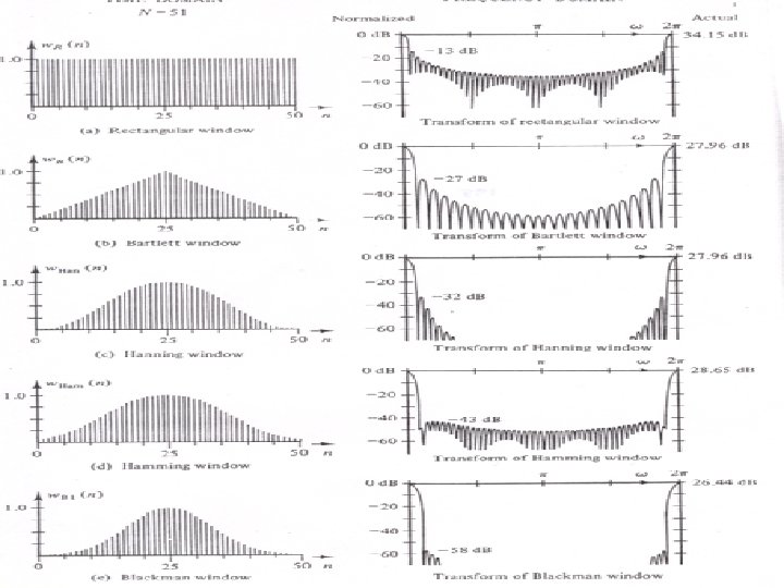
Empirical Mathematic Models Of Different Type Of Windows Window Representation Expression Rectangular w. R[n] 1 Bartlett w. T[n] 1 – {2|n| / (N-1)} Von Hann whn [n] 0. 50 + 0. 50 cos{2 n /(N-1)} Hamming whm [n] 0. 54 + 0. 46 cos{2 n /(N-1)} Blackman wb [n] 0. 42 +0. 50 cos{2 n /(N-1)} +0. 08 cos{4 n /(N-1)} Kaiser w. K[n, ] Io(x 1)/Io(x 2); ratio of modified Bessel’s function of order zero; where x 1=( {1 – 4[n/(N-1)]2}); and x 2= ( )

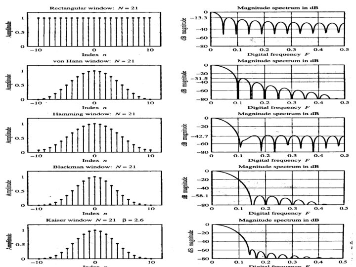
Characteristics of Windows We now examine the characteristics of various other type of windows and compare their performances for N=21 and N=51. Before that note various nomeclatures.

Mathematical representation: Nomenclatures 1. 2. 3. 4. 5. 6. 7. GP / GS = Peak Gain of main-lob / side-lobe d. B ASL = Side-lobe attenuation = (GP /GS) d. B. WM = Half-width of main-lobe W 6 / W 3 = - 6 d. B / -3 d. B half-width DS = stop-band attenuation d. B/dec. FWS = C/N where C= constant of filter. WS = Half width in main-lobe to the peak level of first side lob. 8. Aws= Peak side-lobe attenuation in d. B 9. AWP = Pass band attenuation in d. B

Window Gp GS/Gp ASLd. B WM WS W 6 W 3 DS AWS FWS AWP Rectangular 1 0. 2172 13. 3 1 0. 81 0. 6 0. 44 20 21. 7 0. 92 1. 562 Bartlett Triangular 0. 5 0. 0472 26. 5 2 1. 62 0. 88 0. 63 40 25 Von Hanning 0. 5 0. 0267 31. 5 2 1. 87 1. 0 0. 72 60 44 3. 21 0. 1103 Hamming 0. 54 0. 0073 42. 7 2 1. 91 0. 9 0. 65 20 53 3. 47 0. 0384 Blackman 0. 42 0. 0012 58. 1 3 2. 82 1. 14 0. 82 60 75. 3 5. 71 0. 003 Kaiser = 0. 26 0. 431 4 0. 0010 60 2. 98 2. 72 1. 11 0. 80 20 Note: The widths; WM, WS, W 6, W 3; must be normalized by the window length N. Empirical Values for Kaiser Window depends on the value of defined as: GP = |sinc(j )| / Io( ); WM = (1+ 2); ASL = Sinh( )/0. 22 ; W 6 = (0. 661+ 2)

PROCEDURE OF CALCULATING FILTER COEFFICIENTS USING WINDOW Specify the desired frequency response of the filter Hd( ). Obtain the impulse response h. D [n] of the desired filter by inverse Fourier transform. Select a window which satisfies the passband attenuation specification.

PROCEDURE OF CALCULATING FILTER COEFFICIENTS USING WINDOW… Determine the number of coefficients using the appropriate relationship between the filter length and the transition width f expressed as a fraction of the sampling frequency. Obtain the values of w[n] for the chosen window function and that of the actual FIR coefficients h[n] and multiplying them. Plot the response and verify the compliance of specifications.

convolution of an ideal filter with a sinc window function. Peak side lob a ttenu ation

Comparison of commonly used windows with Kaiser window: Window type Peak Approximate. Appx. normalized Width of peak error side lob main-lob 20 log amplitude Rectangular -13 4 /(M+1) Equivalent Kaiser Window Transition Width -21 0 1. 81 /M Bartlett -25 8 /M -25 1. 33 2/37 /M Hanning -31 8 /M -44 3. 86 5. 01 /M Hamming -41 8 /M -53 4. 86 6/27 /M Blackman -57 12 /M -74 7. 04 9. 19 /M The comparison shows that the Kaiser window is more efficient than any other window in question.

Design using Kaiser Window The filter function is HD( )= 2 f 2 sinc(n 2) -2 f 1 sinc(n 1) Because of stop-band attenuation characteristics, either of the Blackman or, Kaiser windows can be used. From the specifications of pass band stop-band: 20 log(1+ p) = 0. 1 d. B or, p = 0. 0115; -20 log ( s) = 60 d. B, or, s = 0. 001. therefore = min( p, s) = 0. 001. f = transition band width/sampling frequency = 50/1 =0. 05= (AWS-7. 95)/ 14. 36 N = (60 -7. 95)/14. 36 N or, N =72. 49 73.

Design using Kaiser Window… Calculation of by empirical formulae. =0 if A 21 d. B; = 0. 5842(AWS -21)0. 4 + 0. 07886(A-21) if A <21<50 d. B = 0. 1102(AWS -8. 7) if A 50 Hence = 5. 65 Evaluate the coefficients. Evaluate the performance. plot the graph and verify the performance of designed filter.

Advantages and disadvantages of the window method. It is simple to apply and simple to understand. It involves minimum computation. Lacks flexibility. Both peak pass band stopband ripples are nearly equal, limits the choice of designer. Because of convolution of the spectrum of the window function and the desired response, pass band stop-band edge frequencies can not be precisely specified. Maximum ripple magnitudes in pass-band stop-band in the filter response is fixed regardless of N (except in Kaiser Window).