Design by Induction Part 2 Dynamic Programming Bibliography

Design by Induction – Part 2 Dynamic Programming Bibliography: [Manber] – chap 5 [CLRS] – chap 15

Review: Design of algorithms by induction • Induction used in algorithm design: – Base case: Solve a small instance of the problem – Assumption: assume you can solve smaller instances of the problem – Induction step: Show you can construct the solution of the problem from the solution(s) of the smaller problem(s)

Review: Design of algorithms by induction • The inductive step is always based on a reduction from problem size n to problems of size <n. – n -> n-1 or n -> n/2 or n -> n/4, …? • The key here is how to efficiently make the reduction to smaller problems (subproblems): – Sometimes one has to spend some effort to find the suitable element to remove. (see Celebrity Problem) – If the amount of work needed to combine the subproblems is not trivial, reduce by dividing in subproblems of equal size – divide and conquer (see Skyline Problem)

Problem: • We managed to make the reduction of a problem to problems of smaller size (subproblems). • What if some of these subproblems overlap ? (if they contain common subproblems ? )

Dynamic Programming • A technique for designing (optimizing) algorithms • It can be applied to problems that can be decomposed in subproblems, but these subproblems overlap. • Instead of solving the same subproblems repeatedly, applying dynamic programming techniques helps to solve each subproblem just once.

Dynamic Programming Examples • Binomial Coefficients • The Integer Exact Knapsack • Longest Common Subsequence

Binomial Coefficients • The binomial coefficient C(n, k) is the number of ways of choosing a subset of k elements from a set of n elements. • By its definition, C(n, k)=n! / ((n-k)!*k!) • This definition formula is not used for computation because even for small values of n, the values of n factorial n! get really large. • Instead, C(n, k) can be computed by following formula: • C(n, k)=C(n-1, k-1)+C(n-1, k) • C(n, 0)=1 • C(n, n)=1

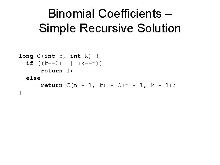
Binomial Coefficients – Simple Recursive Solution long C(int n, int k) { if ((k==0) || (k==n)) return 1; else return C(n - 1, k) + C(n - 1, k - 1); }

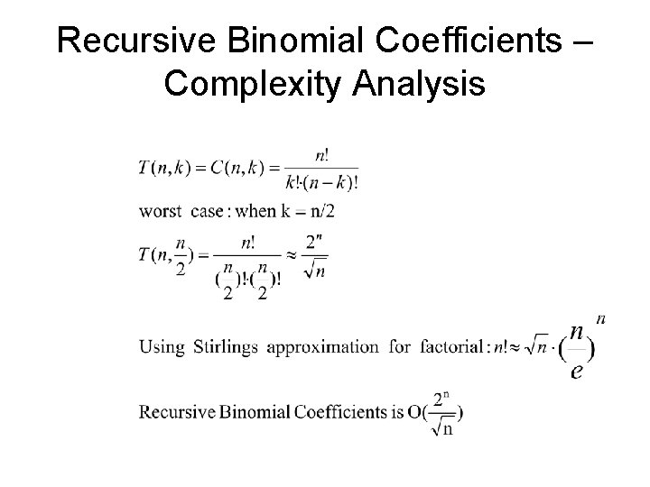
Recursive Binomial Coefficients – Complexity Analysis

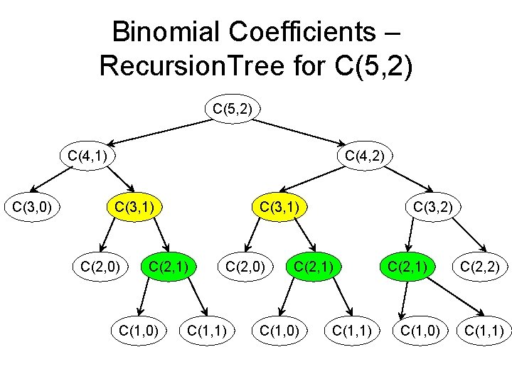
Binomial Coefficients – Recursion. Tree for C(5, 2) C(4, 1) C(3, 0) C(4, 2) C(3, 1) C(2, 0) C(3, 1) C(2, 1) C(1, 0) C(2, 0) C(1, 1) C(3, 2) C(2, 1) C(1, 0) C(1, 1) C(2, 1) C(1, 0) C(2, 2) C(1, 1)

Optimization level 1: Memoization • We can speed up the recursive algorithm by writing down in a table the results of the recursive calls (the subproblems) and looking them up again if we need them later. • In this way we do not compute again a recursive call that was already computed before, just take the result from the table • This process was called memoization – Memoization (not memorization!): the term comes from memo (memorandum), since the technique consists of recording a value so that we can look it up later.

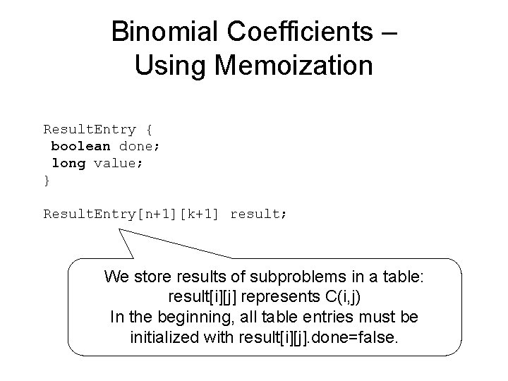
Binomial Coefficients – Using Memoization Result. Entry { boolean done; long value; } Result. Entry[n+1][k+1] result; We store results of subproblems in a table: result[i][j] represents C(i, j) In the beginning, all table entries must be initialized with result[i][j]. done=false.

Binomial Coefficients – Using Memoization (cont) long C(int n, int k) { if (result[n][k]. done == true) return result[n][k]. value; if ((k == 0) || (k == n)) { result[n][k]. done = true; result[n][k]. value = 1; return result[n][k]. value; } result[n][k]. done = true; result[n][k]. value = C(n - 1, k) + C(n - 1, k - 1); return result[n][k]. value; }

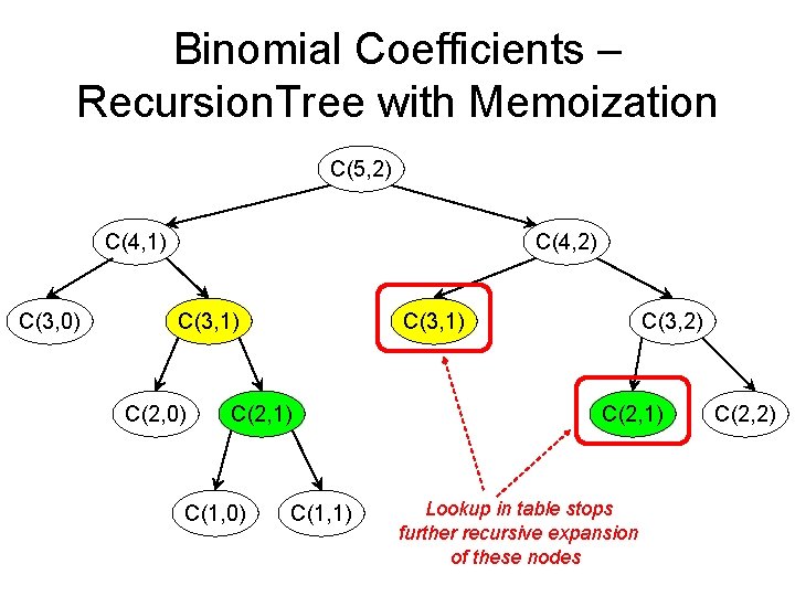
Binomial Coefficients – Recursion. Tree with Memoization C(5, 2) C(4, 1) C(3, 0) C(4, 2) C(3, 1) C(2, 0) C(3, 1) C(2, 1) C(1, 0) C(1, 1) C(3, 2) C(2, 1) Lookup in table stops further recursive expansion of these nodes C(2, 2)

Binomial Coefficients w. Memoization – Complexity Analysis • T(n, k) – exactly n*k table entries are assigned exactly once

Optimization level 2: Dynamic Programming • We want to eliminate recursivity • We look at the recursion tree to see in which order are done the elements of the result table • If we figure out the order, we can replace the recursion with an iterative loop that intentionally fills the table in the right order • This technique is called Dynamic Programming – Dynamic programming: The term was introduced in the 1950 s by Richard Bellman developed methods for constructing training and logistics schedules for the air forces, or as they called them, ‘programs’. The word ‘dynamic’ is meant to suggest that the table is filled in over time, rather than all at once

Binomial Coefficients – Table Filling Order • result[i][j] stores the value of C(i, j) • Table has n+1 rows and k+1 columns, k<=n • Initialization: C(i, 0)=1 and C(i, i)=1 for i=1 to n 0 0 1 1 n 1 1 i 1 1 1 n k 1 1 Entries that must be computed 1 1

Binomial Coefficients – Order (cont) • result[i][j] stores the value of C(i, j) • Rest of entries (i, j), for i=2 to n and j = 1 to i-1 are computed using entry (i-1, j-1) and (i-1, j) 0 0 1 i-1 i n 1 j k n

Binomial Coefficients – Dynamic Programming long[][]result; long C(int n, int k) { result = new long [n + 1]; int i, j; for (i=0; i<=n; i++) { result[i][0]=1; Time: O(n*n) (or O(n*k)) result[i][i]=1; } Memory: O(n*n) (or O(n*k)) for (i=2; i<=n; i++) for(j=1; j<i; j++) result[i][j]=result[i-1][j-1]+result[i-1][j]; return result[n][k]; }

Optimization level 3: Memory Efficient Dynamic Programming • In many dynamic programming algorithms, it may be not necessary to retain all intermediate results through the entire computation. • Every step (every subproblem) depends usually on a reduced set of subproblems, not all other subproblems • We replace the big table storing the results of all subproblems by some smaller buffers that are reused during the computation

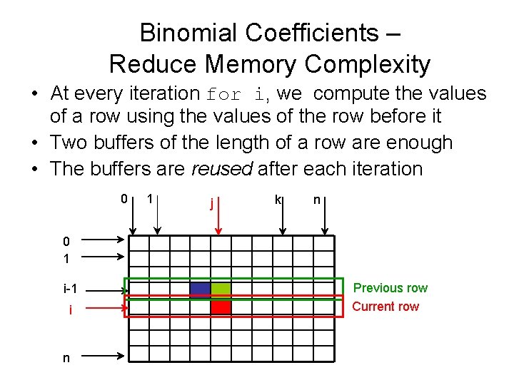
Binomial Coefficients – Reduce Memory Complexity • At every iteration for i, we compute the values of a row using the values of the row before it • Two buffers of the length of a row are enough • The buffers are reused after each iteration 0 1 j k n 0 1 i-1 i n Previous row Current row

Binomial Coefficients – Memory Efficient Dynamic Programming long C(int n, int k) { long[] result 1 = new long[n + 1]; long[] result 2 = new long[n + 1]; result 1[0] = 1; result 1[1] = 1; for (int i = 2; i <= n; i++) { result 2[0] = 1; for (int j = 1; j < i; j++) result 2[j] = result 1[j - 1] + result 1[j]; result 2[i] = 1; long[] auxi = result 1; result 1 = result 2; Time: O(n*n) (or O(n*k)) result 2 = auxi; } Memory: O(n) (or O(k)) return result 1[k]; }

Binomial Coefficients – Example Implementation • • Code for all versions is given in : http: //bigfoot. cs. upt. ro/~ioana/algo/lab_dyn. html The Binomial Coefficients solver interface: – IBinomial. Coef. java The inefficient recursive solution – • The recursive solution based on memoization – • Binomial. Coef. Memoization. java The iterative dynamic programming solution – • Binomial. Coef. Rec. java. Binomial. Coef. Dyn. Prog. java A memory efficient dynamic programming – Binomial. Coef. Dyn. Prog. Mem. Eff. java

Dynamic programming - Summary Dynamic programming as an algorithm design method comprises several optimization levels: 1. Eliminate redundant work on identical subproblems – use a table to store results (memoization) 2. Eliminate recursivity – find out the order in which the elements of the table have to be computed (dynamic programming) 3. Reduce memory complexity if possible

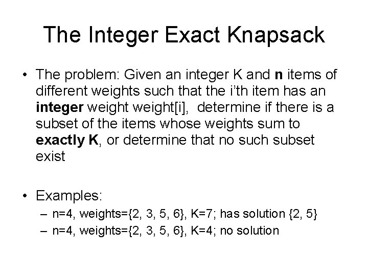
The Integer Exact Knapsack • The problem: Given an integer K and n items of different weights such that the i’th item has an integer weight[i], determine if there is a subset of the items whose weights sum to exactly K, or determine that no such subset exist • Examples: – n=4, weights={2, 3, 5, 6}, K=7; has solution {2, 5} – n=4, weights={2, 3, 5, 6}, K=4; no solution

The Integer Exact Knapsack • The Integer Exact Knapsack problem has 2 versions: – The Simple version, requesting only to find out if there is a solution. – The Complete version, requesting to find out the list of selected items if there is a solution. • We discuss first the Simple version

The Integer Exact Knapsack • Strategy of solving: reduce to smaller subproblems – design by induction • P(n, K) – the problem for n items and a knapsack of K • P(i, k) – the problem for the first i<=n items and a knapsack of size k<=K

The Integer Exact Knapsack (n, K) is If n=1 if weight[n]=K return true else return false If Knapsack(n-1, K)=true return true else if weight[n]=K return true else if K-weight[n]>0 return Knapsack(n-1, K-weight[n]) else return false T(n)= 2*T(n-1)+c, n>2 T(n)=O(2^n)

Knapsack - Recursion tree F(n, K) F(n-1, K) F(n-2, K-s[n-1]) F(n-1, K-s[n]) F(n-2, K-s[n]-s[n-1]) Number of nodes in recursion tree is O(2 n) Max number of distinct function calls F(i, k), where i in [1, n] and k in [1. . K] is n*K F(i, k) returns true if we can fill a sack with size k from the first i items If 2 n >n*K, it is sure that we have 2 n-n*K calls repeated We cannot identify the duplicated nodes in general, they depend on the values of size ! Even if 2 n<n*K, it is possible to have repeated calls, but it depends on the values of size[]

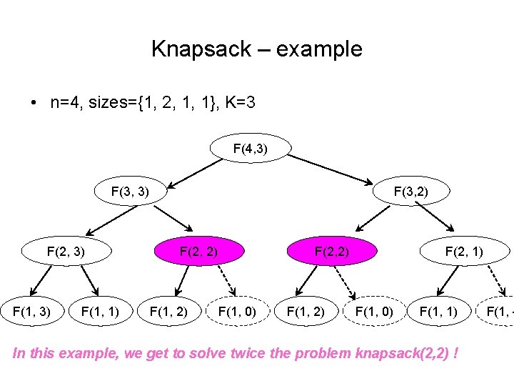
Knapsack – example • n=4, sizes={1, 2, 1, 1}, K=3 F(4, 3) F(3, 3) F(2, 3) F(1, 1) F(3, 2) F(2, 2) F(1, 0) F(1, 2) F(2, 1) F(1, 0) F(1, 1) In this example, we get to solve twice the problem knapsack(2, 2) ! F(1, -

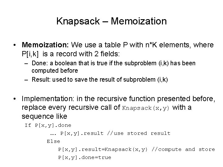
Knapsack – Memoization • Memoization: We use a table P with n*K elements, where P[i, k] is a record with 2 fields: – Done: a boolean that is true if the subproblem (i, k) has been computed before – Result: used to save the result of subproblem (i, k) • Implementation: in the recursive function presented before, replace every recursive call of Knapsack(x, y) with a sequence like If P[x, y]. done …. P[x, y]. result //use stored result Else P[x, y]. result=Knapsack(x, y) //compute and store P[x, y]. done=true

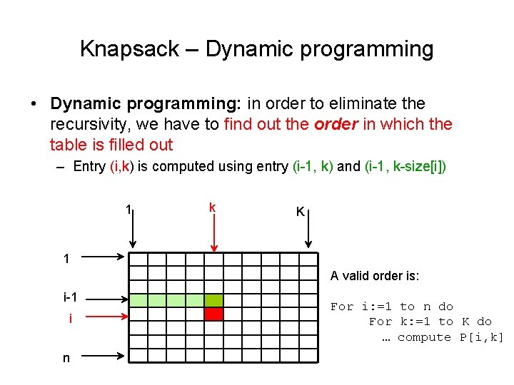
Knapsack – Dynamic programming • Dynamic programming: in order to eliminate the recursivity, we have to find out the order in which the table is filled out – Entry (i, k) is computed using entry (i-1, k) and (i-1, k-size[i]) 1 k K 1 A valid order is: i-1 i n For i: =1 to n do For k: =1 to K do … compute P[i, k]

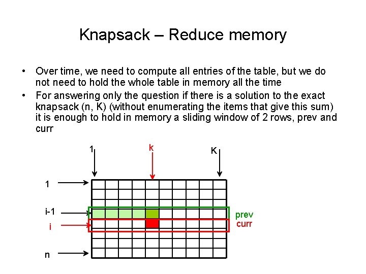
Knapsack – Reduce memory • Over time, we need to compute all entries of the table, but we do not need to hold the whole table in memory all the time • For answering only the question if there is a solution to the exact knapsack (n, K) (without enumerating the items that give this sum) it is enough to hold in memory a sliding window of 2 rows, prev and curr 1 k K 1 i-1 i n prev curr

Knapsack – determine also the set of items • The Complete version of the problem: we are also interested in finding the actual subset that fits in the knapsack • Solution: – we can add to the table entry a flag that indicates whether the corresponding item has been selected in that step – This flag can be traced back from the last entry which is (n, K) and the subset can be recovered

Knapsack – The Complete Version • Reduce the memory complexity in the case of the complete version ? – we can work with 2 row buffers, but we have to add to every row entry also the set of items representing the solution of this subproblem – In the worst case (when all the n items are selected) we use the same memory as with the big table – In the average case (when fewer items are selected) we can use less memory

Knapsack - Homework • Implement the solution of the Knapsack problem (the Simple version) as a memory efficient dynamic programming solution. • Part of Lab 10 – You are given an inefficient recursive implementation for Knapsack. Simple_Recursive. java and its test program – While the given recursive implementation works well for the short set, it will get stack overflow errors for the long set. – A dynamic programming solution using a big table will most likely get out of memory errors for long sets. – Optimize the implementations of the integer exact knapsack solvers such that they can handle long sets of weights !

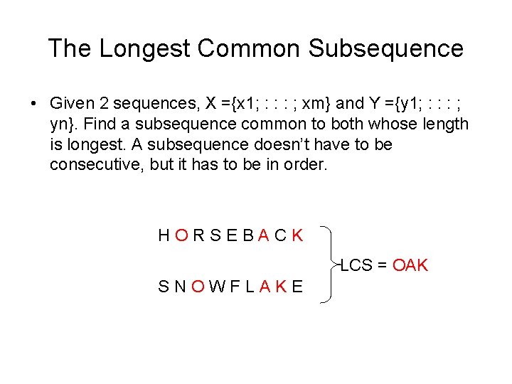
The Longest Common Subsequence • Given 2 sequences, X ={x 1; : : : ; xm} and Y ={y 1; : : : ; yn}. Find a subsequence common to both whose length is longest. A subsequence doesn’t have to be consecutive, but it has to be in order. H O R S E B A C K LCS = OAK S N O W F L A K E

The LCS Problem • The LCS problem has 2 versions: – The Simple version, requesting only to find out the length of the longest common subsequence – The Complete version, requesting to find out the sequence itself • We discuss first the Simple version

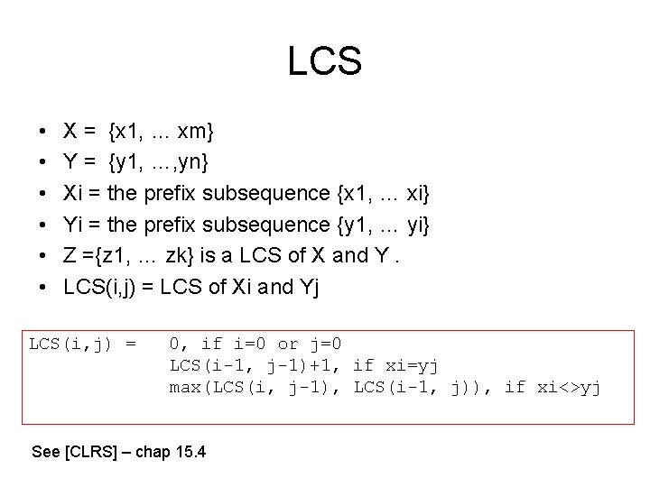
LCS • • • X = {x 1, … xm} Y = {y 1, …, yn} Xi = the prefix subsequence {x 1, … xi} Yi = the prefix subsequence {y 1, … yi} Z ={z 1, … zk} is a LCS of X and Y. LCS(i, j) = LCS of Xi and Yj LCS(i, j) = 0, if i=0 or j=0 LCS(i-1, j-1)+1, if xi=yj max(LCS(i, j-1), LCS(i-1, j)), if xi<>yj See [CLRS] – chap 15. 4

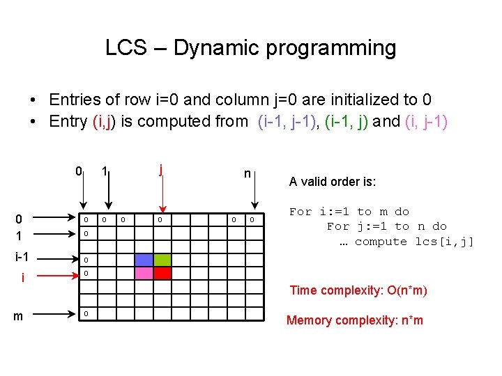
LCS – Dynamic programming • Entries of row i=0 and column j=0 are initialized to 0 • Entry (i, j) is computed from (i-1, j-1), (i-1, j) and (i, j-1) 0 0 1 i-1 j 1 0 0 0 n 0 0 A valid order is: For i: =1 to m do For j: =1 to n do … compute lcs[i, j] 0 i 0 m 0 Time complexity: O(n*m) Memory complexity: n*m

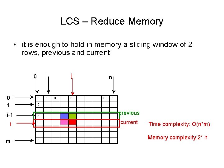
LCS – Reduce Memory • it is enough to hold in memory a sliding window of 2 rows, previous and current 0 0 1 i-1 j 1 0 0 n 0 0 i 0 m 0 previous current Time complexity: O(n*m) Memory complexity: 2* n

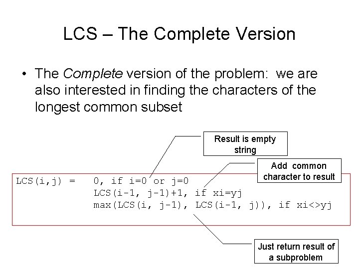
LCS – The Complete Version • The Complete version of the problem: we are also interested in finding the characters of the longest common subset Result is empty string LCS(i, j) = Add common character to result 0, if i=0 or j=0 LCS(i-1, j-1)+1, if xi=yj max(LCS(i, j-1), LCS(i-1, j)), if xi<>yj Just return result of a subproblem

LCS – The Complete Version • We must be able to restore the set of characters that form the LCS • Solution: – we can add to the table entry a “direction field” that points to the subproblem extended by the current problem (one of the 3 possibilities: North, NW, West) – This “direction field” can be traced back from the last entry which is (n, m) and the subset can be recovered – Each “NW” on the direction sequence corresponds to an entry for which the character xi == yj is a member of an LCS

[CLRS – chap 15. 4, page 394]

LCS – Restoring the common sequence [CLRS – chap 15. 4, page 395]

LCS - Example [CLRS – Fig. 15. 8]

LCS – The Complete Version • Is it possible to reduce the memory complexity in the case of the complete version ? – we can work with 2 row buffers, but we have to add to every row entry also the set of items representing the solution of this subproblem – In the worst case (when the strings are equal and the LCS is a string itself) we use the same memory as with the big table – In the average case (when fewer characters are selected) we can use less memory

LCS - Homework • Implement the solution of the LCS problem (the Complete version) as a dynamic programming solution. • Part of Lab 10 – You are given an inefficient recursive implementation for LCS_Complete_Recursive. java and its test program – While the given recursive implementation works well for very short strings (10 characters), it will last very long for a pair of strings of some hundreds characters. – Optimize the implementations of the integer exact knapsack solvers such that they can handle strings of hundreds of characters !

LCS - applications • Molecular biology – DNA sequences (genes) can be represented as sequences of submolecules, each of these being one of the four types: A C G T. In genetics, it is of interest to compute similarities between two DNA sequences by LCS • File comparison – Versioning systems: example - "diff" is used to compare two different versions of the same file, to determine what changes have been made to the file. It works by finding a LCS of the lines of the two files;