Design Analysis of Algorithms Analysis of Algorithms Comparing

Design & Analysis of Algorithms

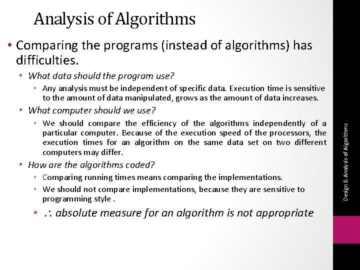
Analysis of Algorithms • Comparing the programs (instead of algorithms) has difficulties. • What data should the program use? • Any analysis must be independent of specific data. Execution time is sensitive to the amount of data manipulated, grows as the amount of data increases. • We should compare the efficiency of the algorithms independently of a particular computer. Because of the execution speed of the processors, the execution times for an algorithm on the same data set on two different computers may differ. • How are the algorithms coded? • Comparing running times means comparing the implementations. • We should not compare implementations, because they are sensitive to programming style. • absolute measure for an algorithm is not appropriate Design & Analysis of Algorithms • What computer should we use?

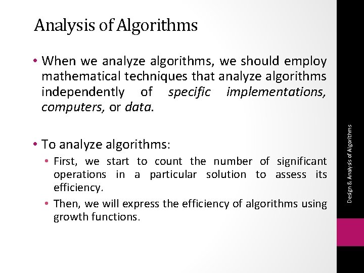
Analysis of Algorithms • To analyze algorithms: • First, we start to count the number of significant operations in a particular solution to assess its efficiency. • Then, we will express the efficiency of algorithms using growth functions. Design & Analysis of Algorithms • When we analyze algorithms, we should employ mathematical techniques that analyze algorithms independently of specific implementations, computers, or data.

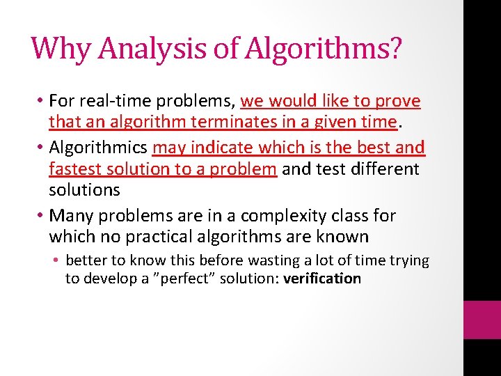
Why Analysis of Algorithms? • For real-time problems, we would like to prove that an algorithm terminates in a given time. • Algorithmics may indicate which is the best and fastest solution to a problem and test different solutions • Many problems are in a complexity class for which no practical algorithms are known • better to know this before wasting a lot of time trying to develop a ”perfect” solution: verification

Analysis of Algorithms • Analysis in the context of algorithms is concerned with predicting the resources that are required: • Computational time • Memory/Space • However, Time – generally measured in terms of the number of steps required to execute an algorithm - is the resource of most interest • By analyzing several candidate algorithms, the most efficient one(s) can be identified

But Computers are So Fast These Days? ? ? • Do we need to bother with algorithmics and complexity any more? • computers are fast, compared to even 10 years ago. . . • Many problems are so computationally demanding that no growth in the power of computing will help very much. • Speed and efficiency are still important

Algorithm Efficiency • There may be several possible algorithms to solve a particular problem • each algorithm has a given efficiency • There are many possible criteria for efficiency • Running time • Space • There always tradeoffs between these two efficiencies

• An array-based list retrieve operation is O(1), a linkedlistbased list retrieve operation is O(n). • But insert and delete operations are much easier on a linkedlist-based list implementation. • When selecting the implementation of an Abstract Data Type (ADT), we have to consider how frequently particular ADT operations occur in a given application. • If the problem size is always very small, we can probably ignore the algorithm’s efficiency. • We have to weigh the trade-offs between an algorithm’s time requirement and its memory requirements. Design & Analysis of Algorithms What is Important?

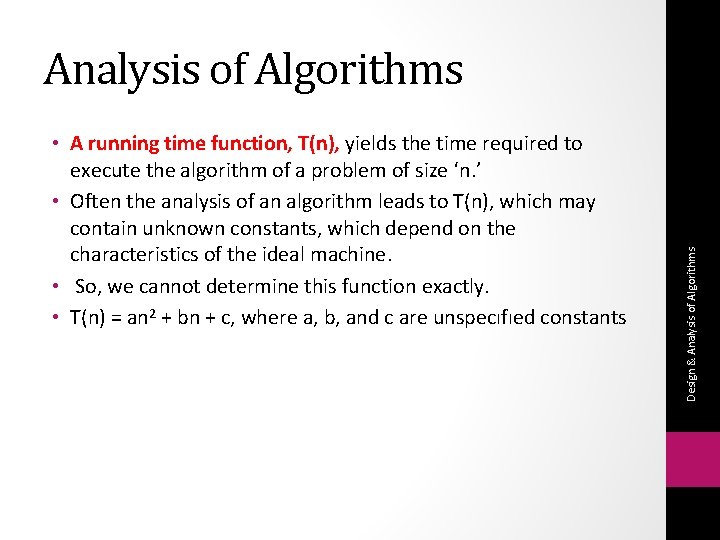
• A running time function, T(n), yields the time required to execute the algorithm of a problem of size ‘n. ’ • Often the analysis of an algorithm leads to T(n), which may contain unknown constants, which depend on the characteristics of the ideal machine. • So, we cannot determine this function exactly. • T(n) = an 2 + bn + c, where a, b, and c are unspecıfıed constants Design & Analysis of Algorithms

Empirical vs Theoretical Analysis • There are two essential approaches to measuring algorithm efficiency: • Empirical analysis • Program the algorithm and measure its running time on example instances • Theoretical analysis • derive a function which relates the running time to the size of instance • In this cousre our focus wiil be on Threoretical analysis.

Advantages of Theory • Theoretical analysis offers some advantages • language independent • not dependent on skill of programmer

Importance of Analyze Algorithm • Need to recognize limitations of various algorithms for solving a problem • Need to understand relationship between problem size and running time • When is a running program not good enough? • Need to learn how to analyze an algorithm's running time without coding it • Need to learn techniques for writing more efficient code • Need to recognize bottlenecks in code as well as which parts of code are easiest to optimize

Why do we analyze about them ? • understand their behavior, and (Job -- Selection, performance, modify( • improve them. (Research (

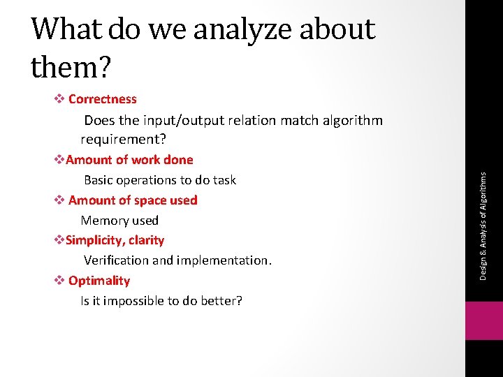
What do we analyze about them? v Correctness v. Amount of work done Basic operations to do task v Amount of space used Memory used v. Simplicity, clarity Verification and implementation. v Optimality Is it impossible to do better? Design & Analysis of Algorithms Does the input/output relation match algorithm requirement?

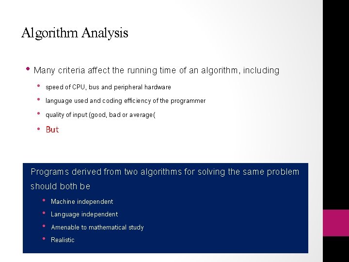
Algorithm Analysis • Many criteria affect the running time of an algorithm, including • speed of CPU, bus and peripheral hardware • language used and coding efficiency of the programmer • quality of input (good, bad or average( • But Programs derived from two algorithms for solving the same problem should both be • • Machine independent Language independent Amenable to mathematical study Realistic

Analysis of Algorithms (assumptions) • Analysis is performed with respect to a computational model • To analyze the algorithm, a computational model should also be determined. • RAM (Random Access Machine) is used for the purpose.

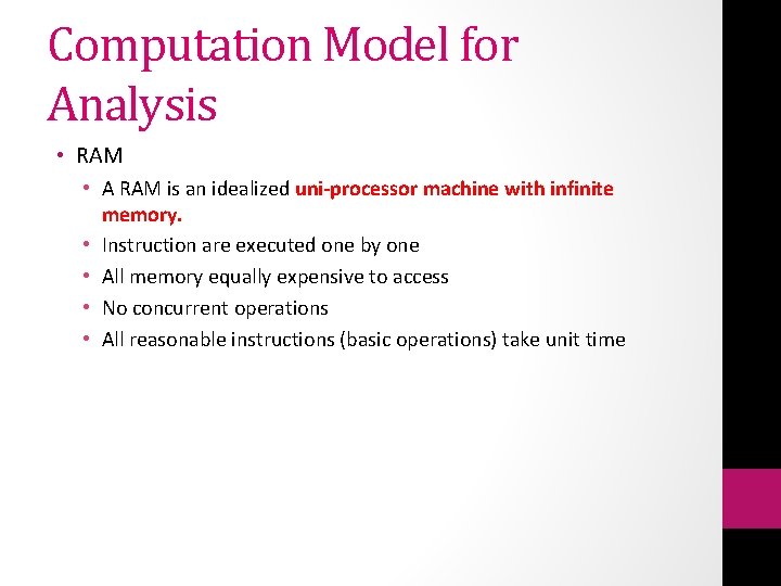
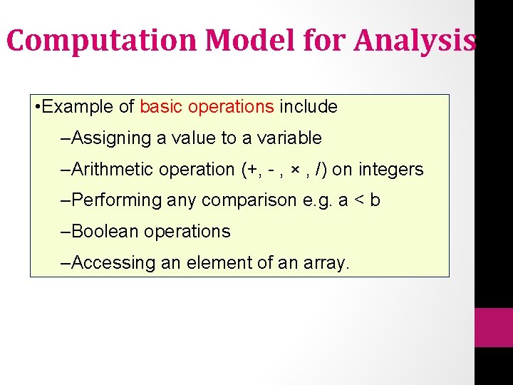
Computation Model for Analysis • RAM • A RAM is an idealized uni-processor machine with infinite memory. • Instruction are executed one by one • All memory equally expensive to access • No concurrent operations • All reasonable instructions (basic operations) take unit time

Computation Model for Analysis • Example of basic operations include –Assigning a value to a variable –Arithmetic operation (+, - , × , /) on integers –Performing any comparison e. g. a < b –Boolean operations –Accessing an element of an array.

Model of Computation (Assumptions) • As we evaluate a new algorithm by comparing its performance with that of previous approaches • Comparisons are asymtotic analyses of classes of algorithms • In theoretical analysis, computational complexity • Estimated in asymptotic sense, i. e. estimating for large inputs • Big O, Omega, Theta etc. notations are used to compute the complexity • Asymptotic notations are used because different implementations of algorithm may differ in efficiency

Analysis • Worst case • Provides an upper bound on running time • An absolute guarantee • Average case • Provides the expected running time • Very useful, but treat with care: what is “average”? • Random (equally likely) inputs • Real-life inputs

Complexity • The complexity of an algorithm is simply the amount of work the algorithm performs to complete its task.

Complexity • Complexity is a function T(n) which measures the time or space used by an algorithm with respect to the input size n. • The running time of an algorithm on a particular input is determined by the number of “Elementary Operations” executed.

What is an Elementary Operation? • An elementary operation is an operation which takes constant time regardless of problem size. • The point is that we can now measure running time in terms of number of elementary operations.

Elementary Operations • Some operations are always elementary • variable assignment • testing if a number is negative • Many can be assumed to be elementary. . • addition, subtraction

Things to Remember in Analysis • Constants or low-order terms are ignore e. g. if f(n) = 2 n 2 then f(n) = O(n 2( • Parameter N, usually referring to number of data items processed, affects running time most significantly. • Worst case is amount of time program would take with worst possible input configuration • worst case is upper bound for input and easier to find. • Average case is amount of time a program is expected to take using "typical" input data • definition of "average" can affect results • average case is much harder to compute • Best case is amount of time program would take with best possible input configuration • best case is lower bound for input.

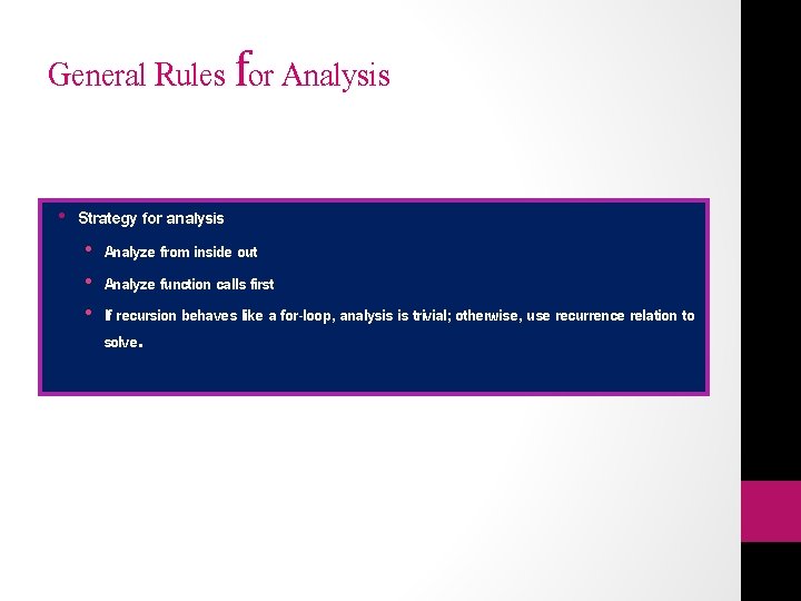
General Rules for Analysis • Strategy for analysis • Analyze from inside out • Analyze function calls first • If recursion behaves like a for-loop, analysis is trivial; otherwise, use recurrence relation to solve.

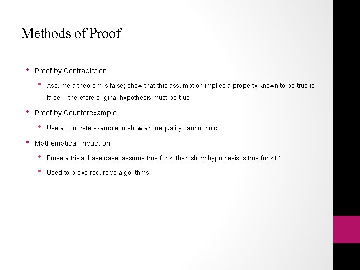
Methods of Proof • Proof by Contradiction • Assume a theorem is false; show that this assumption implies a property known to be true is false -- therefore original hypothesis must be true • Proof by Counterexample • Use a concrete example to show an inequality cannot hold • Mathematical Induction • Prove a trivial base case, assume true for k, then show hypothesis is true for k+1 • Used to prove recursive algorithms

Complexity and Input Size • Complexity is a function that express relationship between time and input size • We are not so much interested in the time and space complexity for small inputs rather the function is only calculated for large inputs.

Complexity-Growth of funtion • The growth of the complexity functions is what is more important for the analysis. • The growth of time and space complexity with increasing input size n is a suitable measure for the comparison of algorithms.

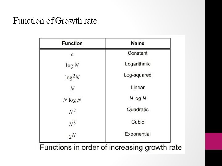
Function of Growth rate

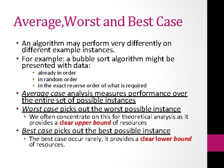
Average, Worst and Best Case • An algorithm may perform very differently on different example instances. • For example: a bubble sort algorithm might be presented with data: • already in order • in random order • in the exact reverse order of what is required • Average case analysis measures performance over the entire set of possible instances • Worst case picks out the worst possible instance • We often concentrate on this for theoretical analysis as it provides a clear upper bound of resources • Best case picks out the best possible instance • The best case occur rarely, it provides a clear lower bound of resources.

Average Case Analysis • Average case analysis can be difficult in practice • to do a realistic analysis we need to know the likely distribution of instances • However, it is often very useful and more relevant than worst case • for example quicksort has a catastrophic (extremly harmful) worst case, but in practice it is one of the best sorting algorithms known

Components of an Algorithm • Sequences • Selections • Repetitions

Sequence • A linear sequence of elementary operations is also performed in constant time. • More generally, given two program fragments P 1 and P 2 which run sequentially in times t 1 and t 2 • we can use the maximum rule which states that the larger time dominates • Complexity will be max(t 1, t 2)

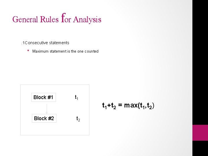
General Rules for Analysis. 1 Consecutive statements • Maximum statement is the one counted Block #1 t 1+t 2 = max(t 1, t 2) Block #2 t 2

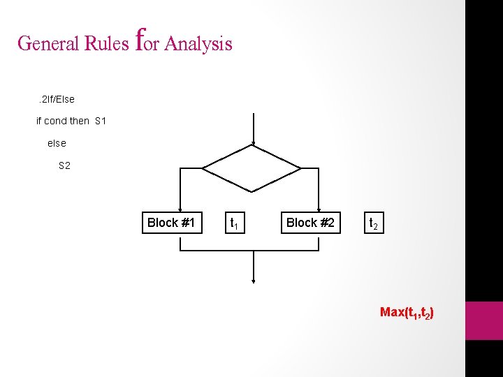
Selection • If <test> then P 1 else P 2 structures are a little harder; conditional loops. • The maximum rule can be applied here too: • max(t 1, t 2), assuming t 1, t 2 are times of P 1, P 2 • However, the maximum rule may prove too conservative • if <test> is always true the time is t 1 • if <test> is always false the time is t 2

General Rules for Analysis. 2 If/Else if cond then S 1 else S 2 Block #1 t 1 Block #2 t 2 Max(t 1, t 2)

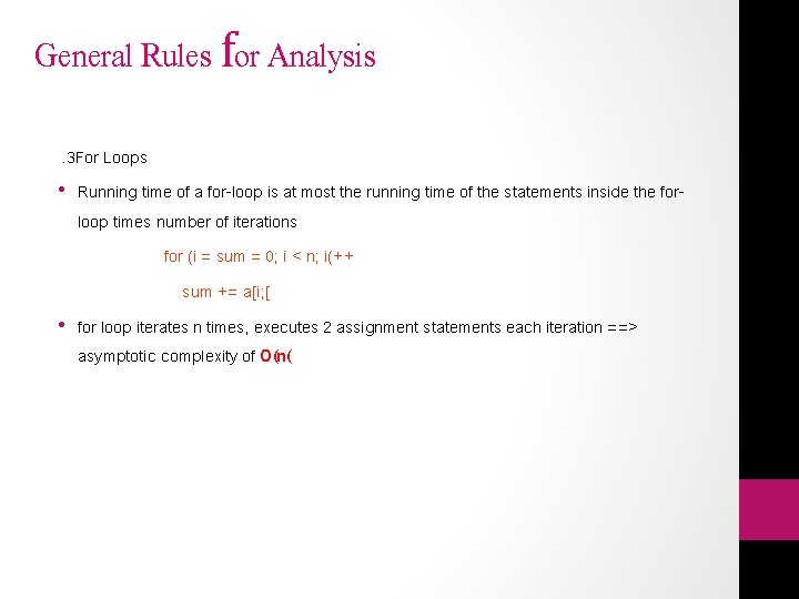
General Rules for Analysis. 3 For Loops • Running time of a for-loop is at most the running time of the statements inside the forloop times number of iterations for (i = sum = 0; i < n; i(++ sum += a[i; [ • for loop iterates n times, executes 2 assignment statements each iteration ==> asymptotic complexity of O(n(

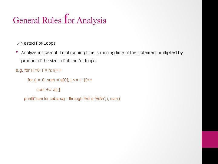
General Rules for Analysis. 4 Nested For-Loops • Analyze inside-out. Total running time is running time of the statement multiplied by product of the sizes of all the for-loops e. g. for (i =0; i < n; i(++ for (j = 0, sum = a[0]; j <= i ; j(++ sum += a[j; [ printf("sum for subarray - through %d is %dn", i, sum; (

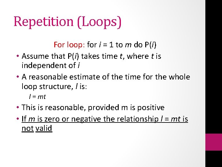
Repetition (Loops) For loop: for i = 1 to m do P(i) • Assume that P(i) takes time t, where t is independent of i • A reasonable estimate of the time for the whole loop structure, l is: l = mt • This is reasonable, provided m is positive • If m is zero or negative the relationship l = mt is not valid

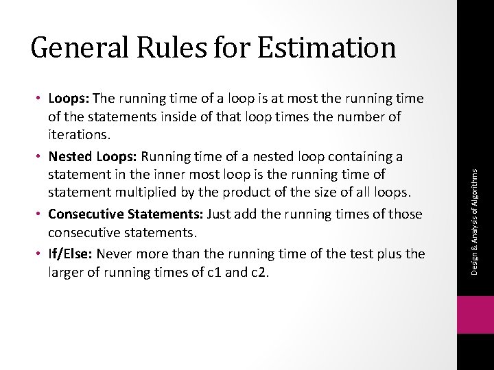
• Loops: The running time of a loop is at most the running time of the statements inside of that loop times the number of iterations. • Nested Loops: Running time of a nested loop containing a statement in the inner most loop is the running time of statement multiplied by the product of the size of all loops. • Consecutive Statements: Just add the running times of those consecutive statements. • If/Else: Never more than the running time of the test plus the larger of running times of c 1 and c 2. Design & Analysis of Algorithms General Rules for Estimation

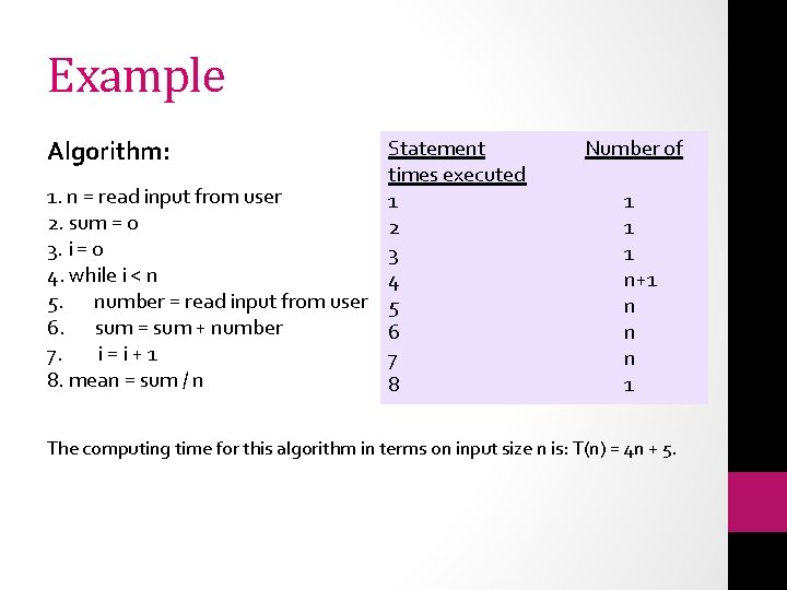
Example Algorithm: Statement times executed 1. n = read input from user 1 2. sum = 0 2 3. i = 0 3 4. while i < n 4 5. number = read input from user 5 6. sum = sum + number 6 7. i=i+1 7 8. mean = sum / n 8 Number of 1 1 1 n+1 n n n 1 The computing time for this algorithm in terms on input size n is: T(n) = 4 n + 5.

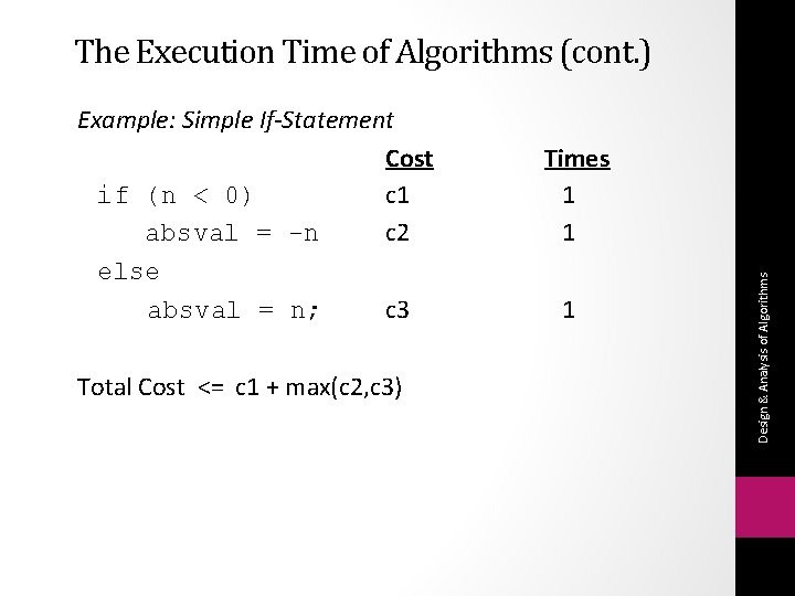
The Execution Time of Algorithms (cont. ) Total Cost <= c 1 + max(c 2, c 3) Times 1 1 1 Design & Analysis of Algorithms Example: Simple If-Statement Cost if (n < 0) c 1 absval = -n c 2 else absval = n; c 3

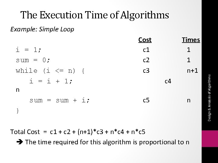
The Execution Time of Algorithms Example: Simple Loop Times 1 1 n+1 c 4 c 5 n Total Cost = c 1 + c 2 + (n+1)*c 3 + n*c 4 + n*c 5 The time required for this algorithm is proportional to n Design & Analysis of Algorithms i = 1; sum = 0; while (i <= n) { i = i + 1; n sum = sum + i; } Cost c 1 c 2 c 3

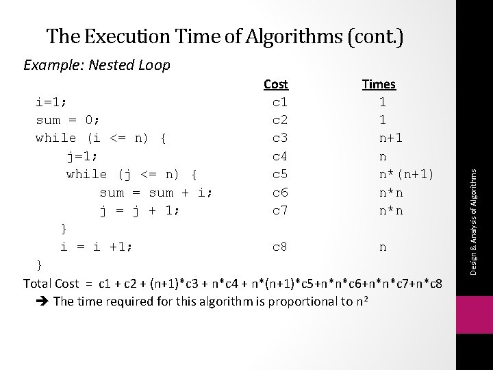
The Execution Time of Algorithms (cont. ) Cost c 1 c 2 c 3 c 4 c 5 c 6 c 7 Times 1 1 n+1 n n*(n+1) n*n i=1; sum = 0; while (i <= n) { j=1; while (j <= n) { sum = sum + i; j = j + 1; } i = i +1; c 8 n } Total Cost = c 1 + c 2 + (n+1)*c 3 + n*c 4 + n*(n+1)*c 5+n*n*c 6+n*n*c 7+n*c 8 The time required for this algorithm is proportional to n 2 Design & Analysis of Algorithms Example: Nested Loop

• EXACT answers are great when we find them; there is something very satisfying about complete knowledge. But there is also a time when approximations are in order. If we run into sum or a recurrence whose solution is not in closed form , we still would like to know something about the answer. Design & Analysis of Algorithms Asymptotic Analysis

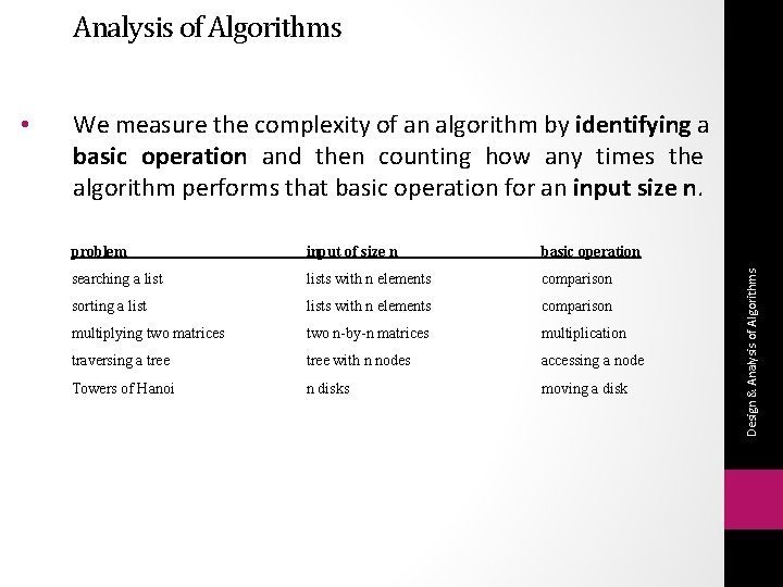
Analysis of Algorithms We measure the complexity of an algorithm by identifying a basic operation and then counting how any times the algorithm performs that basic operation for an input size n. problem input of size n basic operation searching a lists with n elements comparison sorting a lists with n elements comparison multiplying two matrices two n-by-n matrices multiplication traversing a tree with n nodes accessing a node Towers of Hanoi n disks moving a disk Design & Analysis of Algorithms •

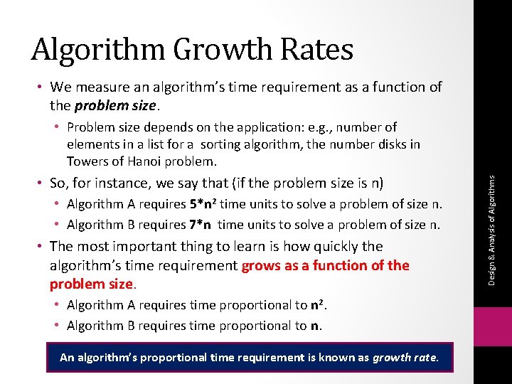
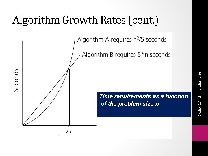
Algorithm Growth Rates • We measure an algorithm’s time requirement as a function of the problem size. • So, for instance, we say that (if the problem size is n) • Algorithm A requires 5*n 2 time units to solve a problem of size n. • Algorithm B requires 7*n time units to solve a problem of size n. • The most important thing to learn is how quickly the algorithm’s time requirement grows as a function of the problem size. • Algorithm A requires time proportional to n 2. • Algorithm B requires time proportional to n. An algorithm’s proportional time requirement is known as growth rate. Design & Analysis of Algorithms • Problem size depends on the application: e. g. , number of elements in a list for a sorting algorithm, the number disks in Towers of Hanoi problem.

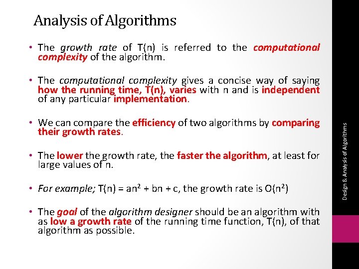
Analysis of Algorithms • The growth rate of T(n) is referred to the computational complexity of the algorithm. • We can compare the efficiency of two algorithms by comparing their growth rates. • The lower the growth rate, the faster the algorithm, at least for large values of n. • For example; T(n) = an 2 + bn + c, the growth rate is O(n 2) • The goal of the algorithm designer should be an algorithm with as low a growth rate of the running time function, T(n), of that algorithm as possible. Design & Analysis of Algorithms • The computational complexity gives a concise way of saying how the running time, T(n), varies with n and is independent of any particular implementation.

Time requirements as a function of the problem size n Design & Analysis of Algorithms Algorithm Growth Rates (cont. )

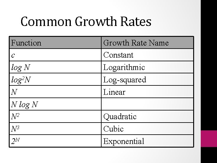
Common Growth Rates Function c log N log 2 N N N log N N 2 N 3 2 N Growth Rate Name Constant Logarithmic Log-squared Linear Quadratic Cubic Exponential

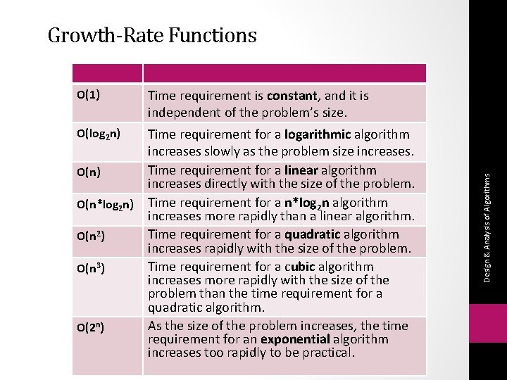
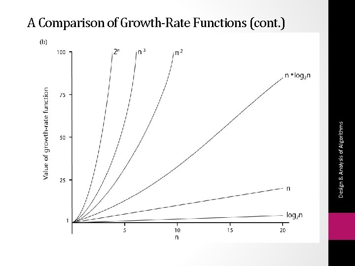
O(1) Time requirement is constant, and it is independent of the problem’s size. O(log 2 n) Time requirement for a logarithmic algorithm increases slowly as the problem size increases. Time requirement for a linear algorithm increases directly with the size of the problem. Time requirement for a n*log 2 n algorithm increases more rapidly than a linear algorithm. Time requirement for a quadratic algorithm increases rapidly with the size of the problem. Time requirement for a cubic algorithm increases more rapidly with the size of the problem than the time requirement for a quadratic algorithm. As the size of the problem increases, the time requirement for an exponential algorithm increases too rapidly to be practical. O(n) O(n*log 2 n) O(n 2) O(n 3) O(2 n) Design & Analysis of Algorithms Growth-Rate Functions

Design & Analysis of Algorithms A Comparison of Growth-Rate Functions (cont. )

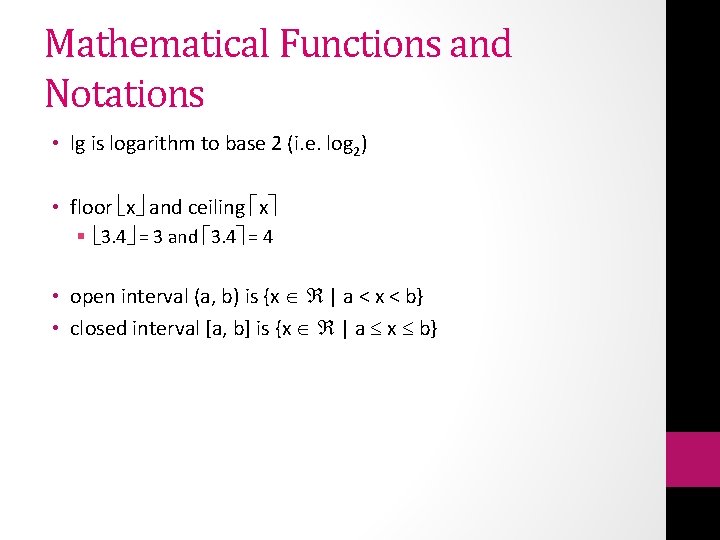
Mathematical Functions and Notations • lg is logarithm to base 2 (i. e. log 2) • floor x and ceiling x § 3. 4 = 3 and 3. 4 = 4 • open interval (a, b) is {x | a < x < b} • closed interval [a, b] is {x | a x b}

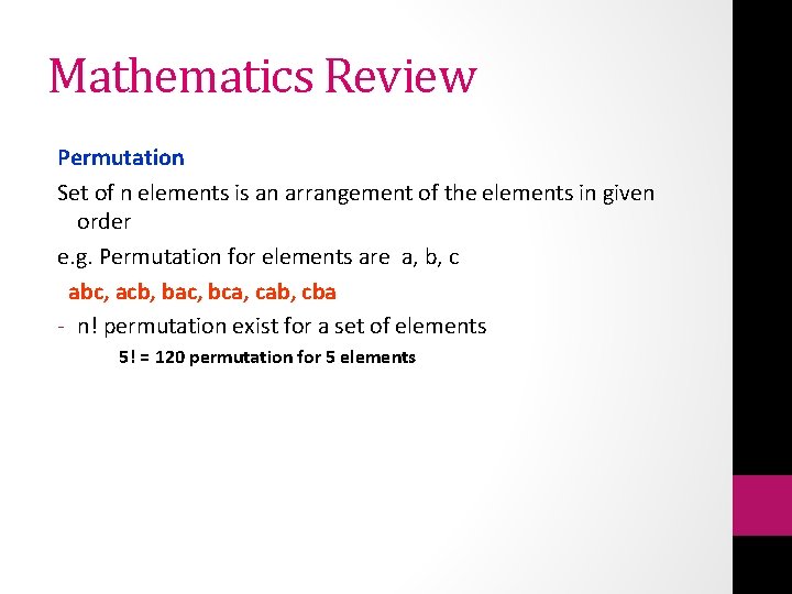
Mathematics Review Permutation Set of n elements is an arrangement of the elements in given order e. g. Permutation for elements are a, b, c abc, acb, bac, bca, cab, cba - n! permutation exist for a set of elements 5! = 120 permutation for 5 elements

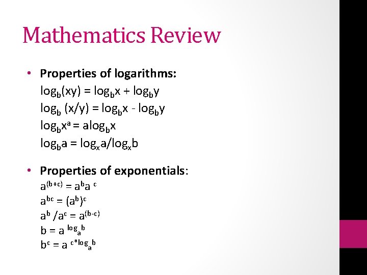
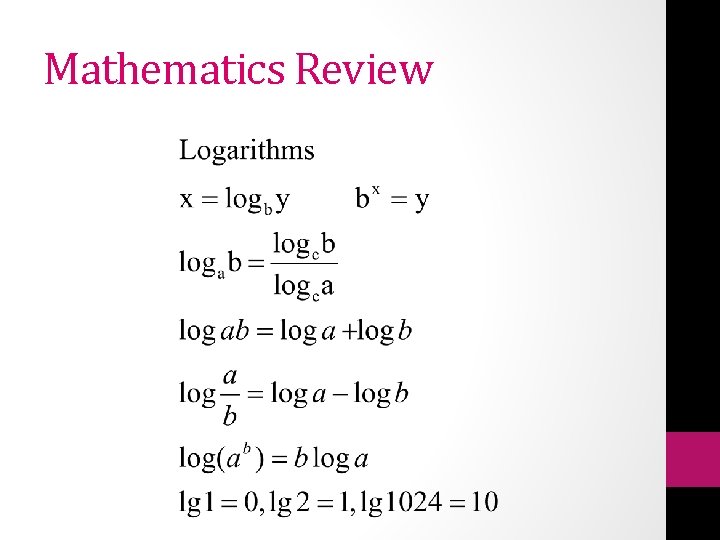
Mathematics Review • Properties of logarithms: logb(xy) = logbx + logby logb (x/y) = logbx - logby logbxa = alogbx logba = logxa/logxb • Properties of exponentials: a(b+c) = aba c abc = (ab)c ab /ac = a(b-c) b = a logab bc = a c*logab

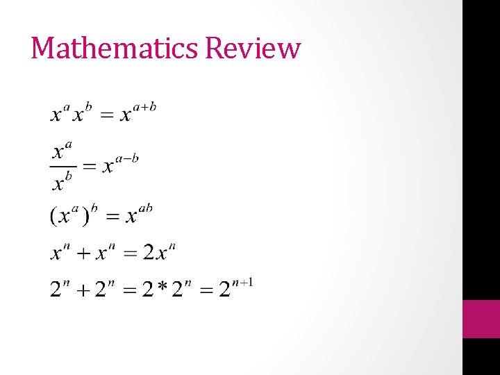
Mathematics Review

Mathematics Review