Descriptors Local features main components 1 Detection Identify
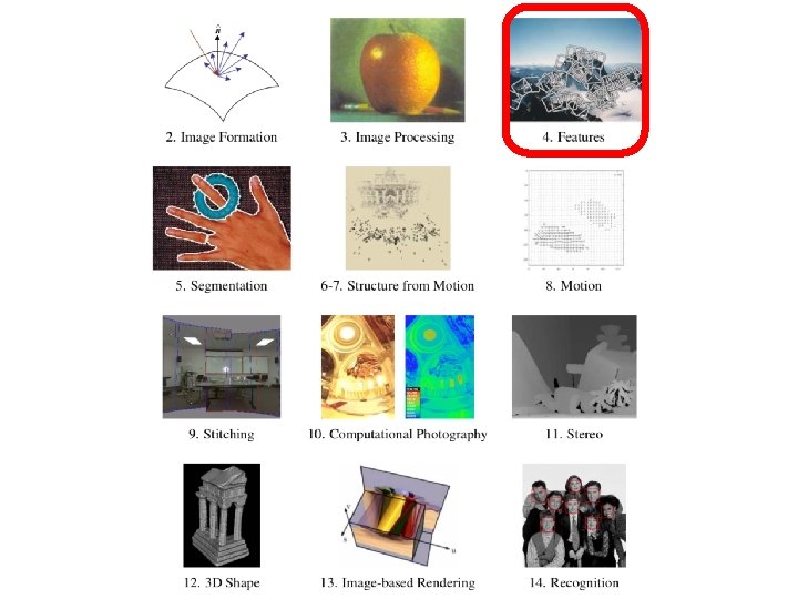
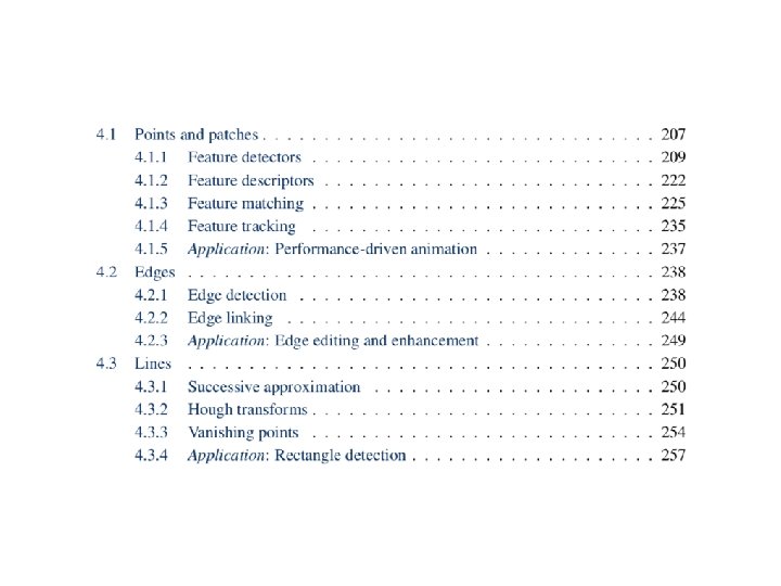
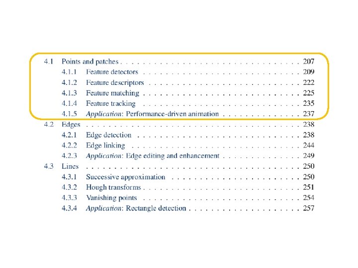


- Slides: 37


Descriptors

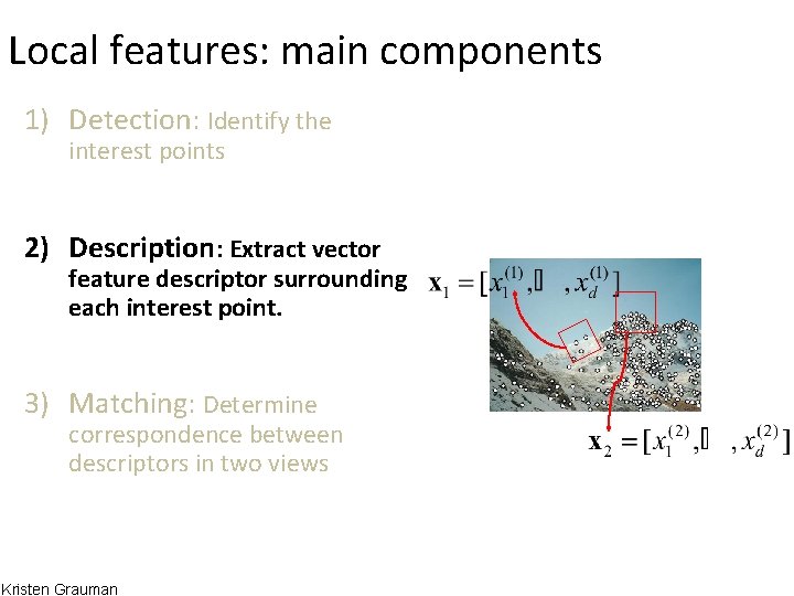
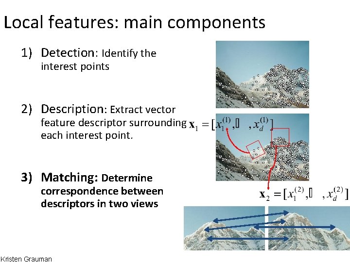
Local features: main components 1) Detection: Identify the interest points 2) Description: Extract vector feature descriptor surrounding each interest point. 3) Matching: Determine correspondence between descriptors in two views Kristen Grauman

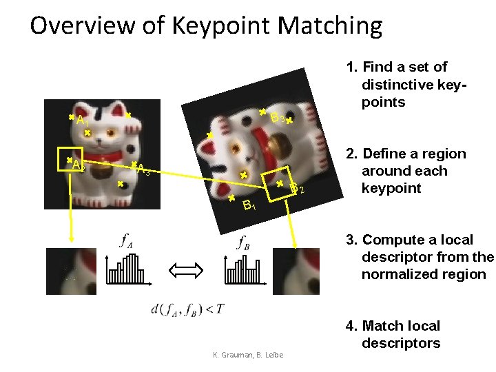
Overview of Keypoint Matching 1. Find a set of distinctive keypoints B 3 A 1 A 2 A 3 B 2 2. Define a region around each keypoint B 1 3. Compute a local descriptor from the normalized region K. Grauman, B. Leibe 4. Match local descriptors

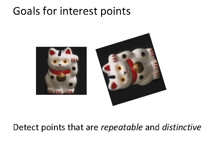
Goals for interest points Detect points that are repeatable and distinctive

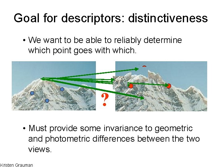
Goal for descriptors: distinctiveness • We want to be able to reliably determine which point goes with which. ? • Must provide some invariance to geometric and photometric differences between the two views. Kristen Grauman

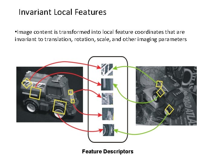
Invariant Local Features • Image content is transformed into local feature coordinates that are invariant to translation, rotation, scale, and other imaging parameters Feature Descriptors

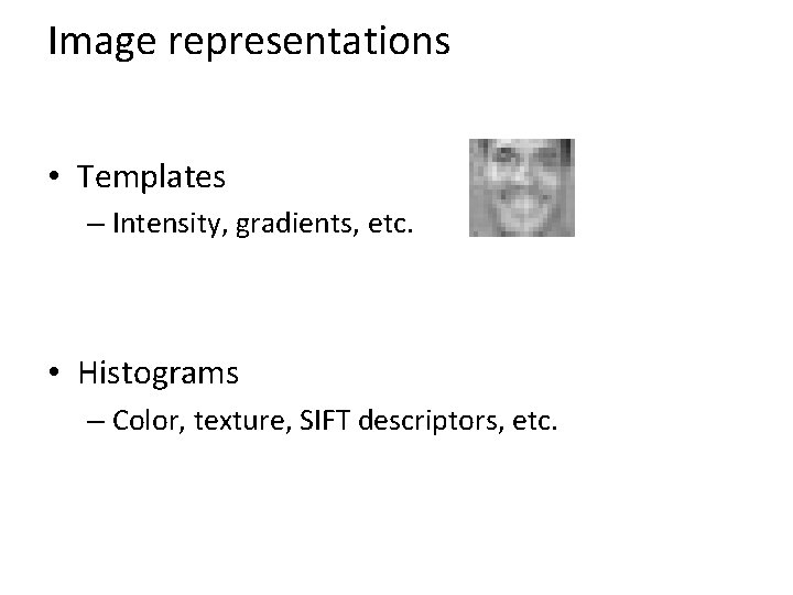
Image representations • Templates – Intensity, gradients, etc. • Histograms – Color, texture, SIFT descriptors, etc.

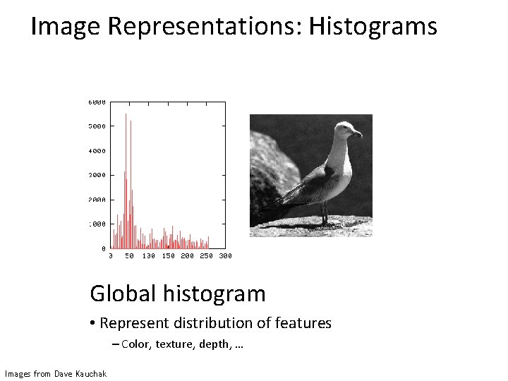
Image Representations: Histograms Global histogram • Represent distribution of features – Color, texture, depth, … Images from Dave Kauchak Space Shuttle Cargo Bay

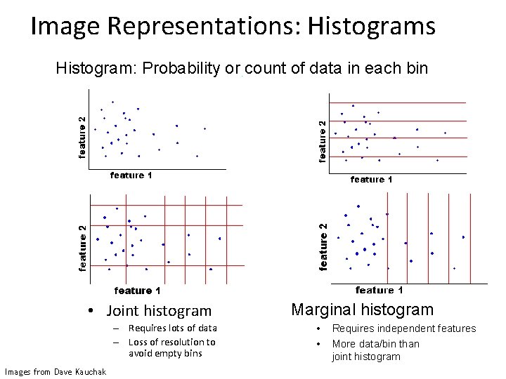
Image Representations: Histograms Histogram: Probability or count of data in each bin • Joint histogram – Requires lots of data – Loss of resolution to avoid empty bins Images from Dave Kauchak Marginal histogram • • Requires independent features More data/bin than joint histogram

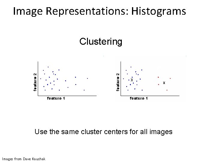
Image Representations: Histograms Clustering EASE Truss Assembly Use the same cluster centers for all images Space Shuttle Cargo Bay Images from Dave Kauchak

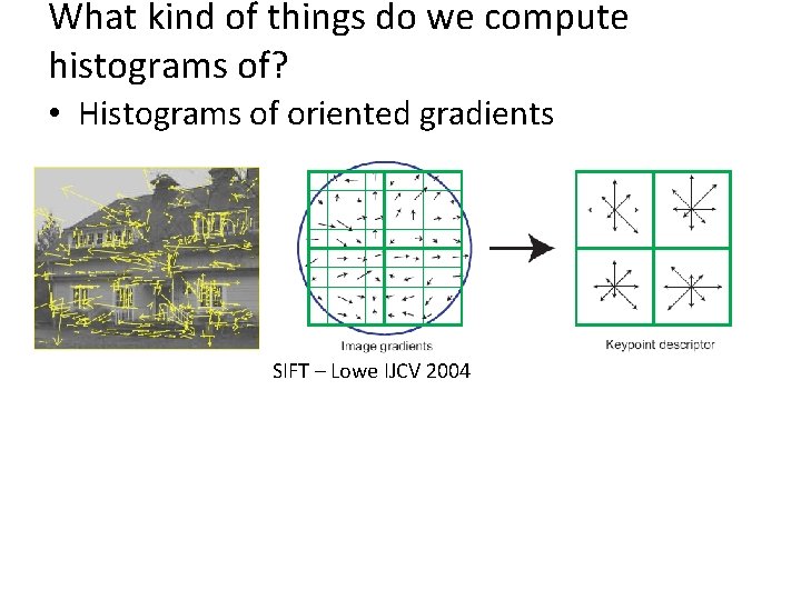
What kind of things do we compute histograms of? • Histograms of oriented gradients SIFT – Lowe IJCV 2004

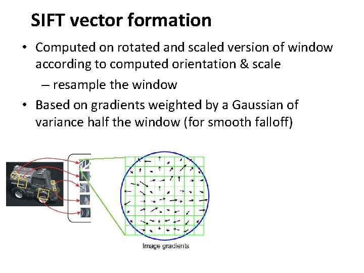
SIFT vector formation • Computed on rotated and scaled version of window according to computed orientation & scale – resample the window • Based on gradients weighted by a Gaussian of variance half the window (for smooth falloff)

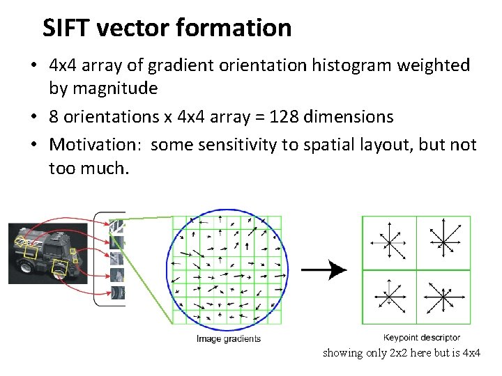
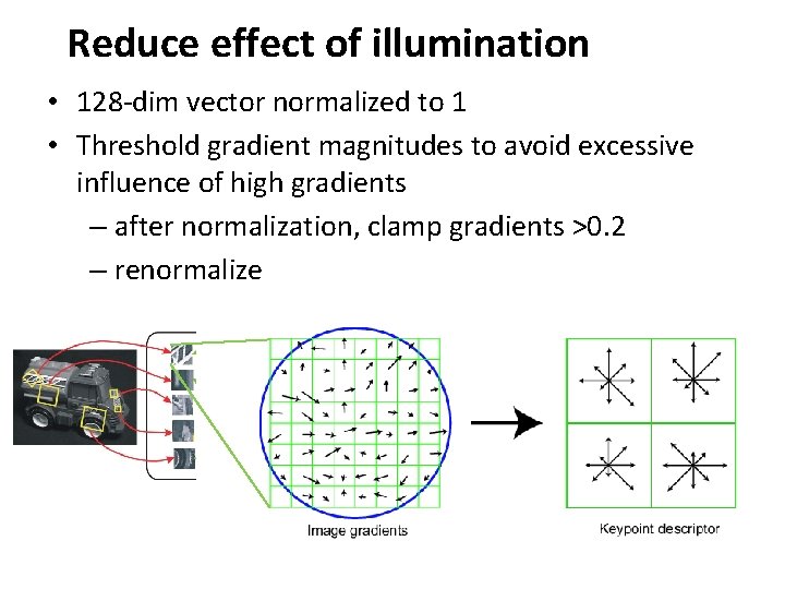
SIFT vector formation • 4 x 4 array of gradient orientation histogram weighted by magnitude • 8 orientations x 4 x 4 array = 128 dimensions • Motivation: some sensitivity to spatial layout, but not too much. showing only 2 x 2 here but is 4 x 4

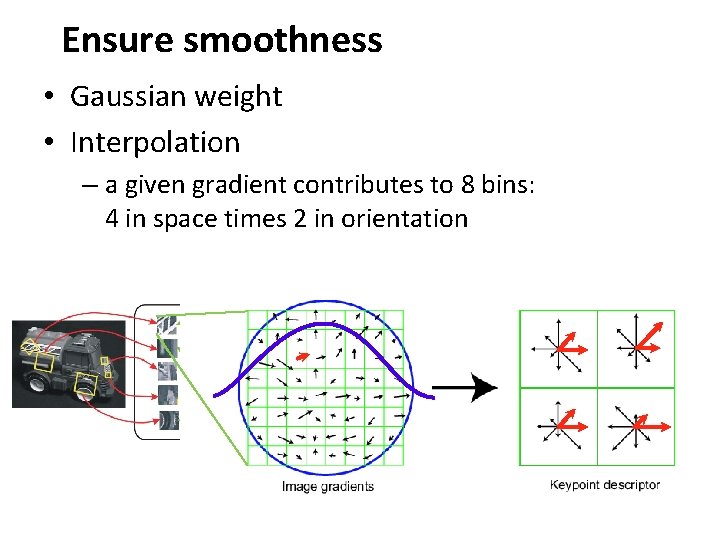
Ensure smoothness • Gaussian weight • Interpolation – a given gradient contributes to 8 bins: 4 in space times 2 in orientation

Reduce effect of illumination • 128 -dim vector normalized to 1 • Threshold gradient magnitudes to avoid excessive influence of high gradients – after normalization, clamp gradients >0. 2 – renormalize

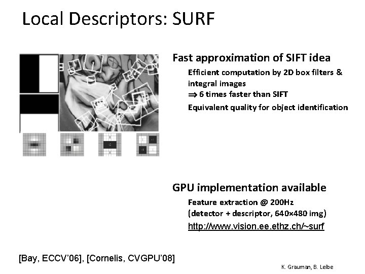
Local Descriptors: SURF • Fast approximation of SIFT idea Ø Ø Efficient computation by 2 D box filters & integral images 6 times faster than SIFT Equivalent quality for object identification • GPU implementation available Ø Ø [Bay, ECCV’ 06], [Cornelis, CVGPU’ 08] Feature extraction @ 200 Hz (detector + descriptor, 640× 480 img) http: //www. vision. ee. ethz. ch/~surf K. Grauman, B. Leibe

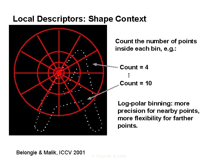
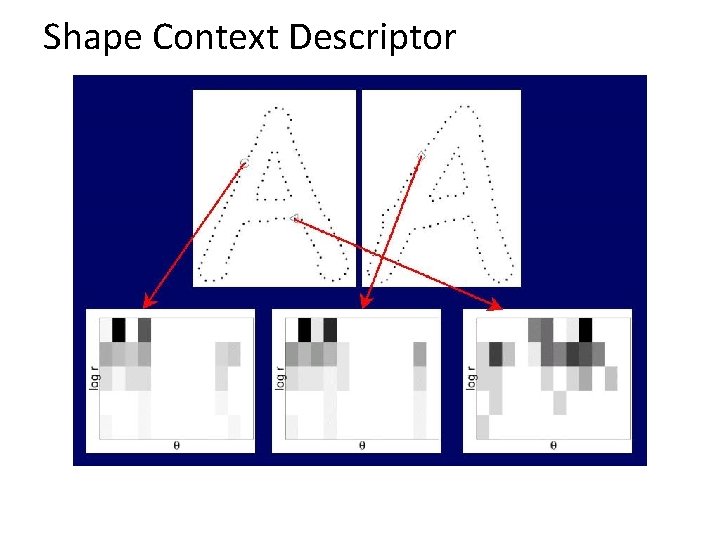
Local Descriptors: Shape Context Count the number of points inside each bin, e. g. : Count = 4. . . Count = 10 Log-polar binning: more precision for nearby points, more flexibility for farther points. Belongie & Malik, ICCV 2001 K. Grauman, B. Leibe

Shape Context Descriptor

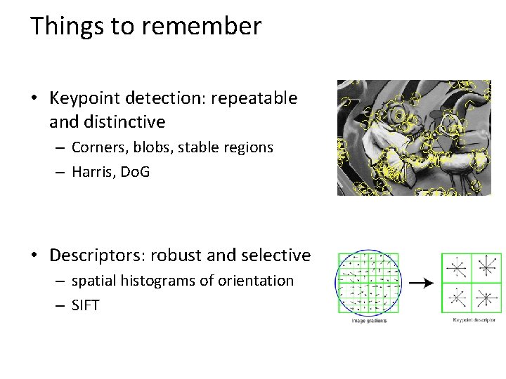
Things to remember • Keypoint detection: repeatable and distinctive – Corners, blobs, stable regions – Harris, Do. G • Descriptors: robust and selective – spatial histograms of orientation – SIFT

Deep Descriptors

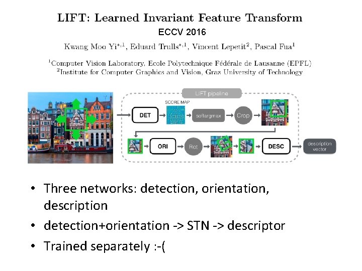
ECCV 2016 • Three networks: detection, orientation, description • detection+orientation -> STN -> descriptor • Trained separately : -(

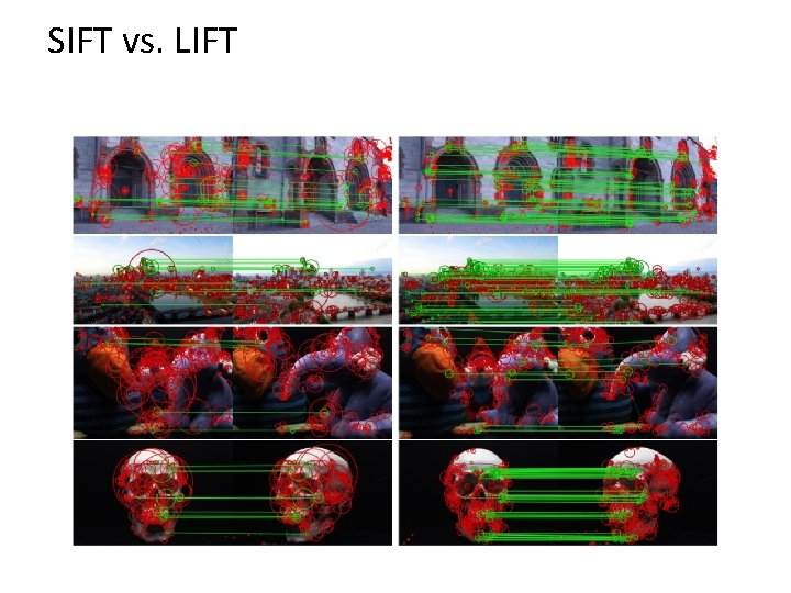
SIFT vs. LIFT

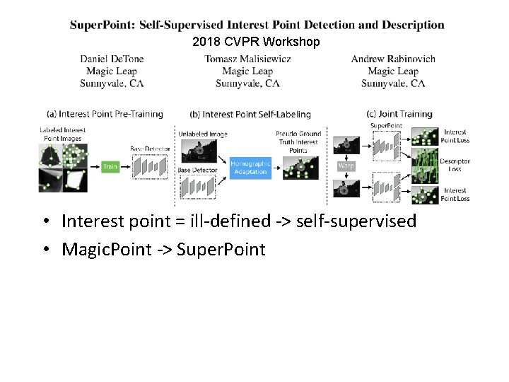
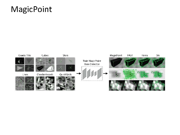
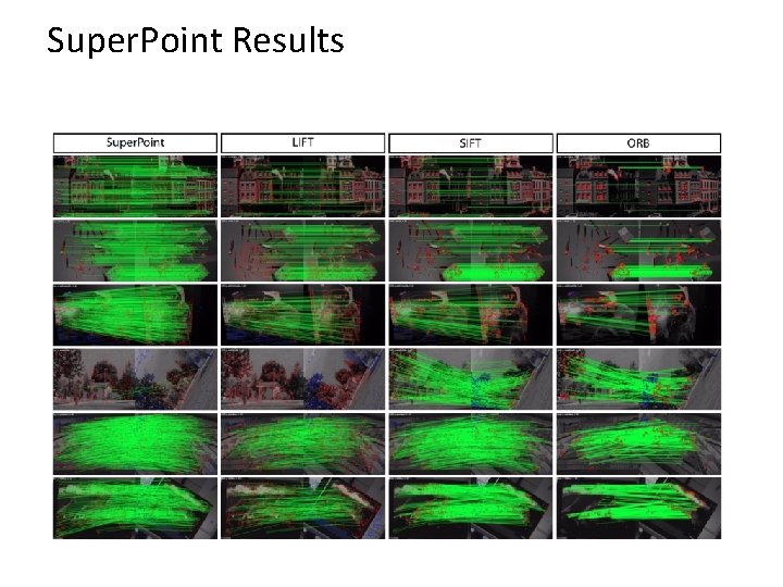
2018 CVPR Workshop • Interest point = ill-defined -> self-supervised • Magic. Point -> Super. Point

Magic. Point

Super. Point Results

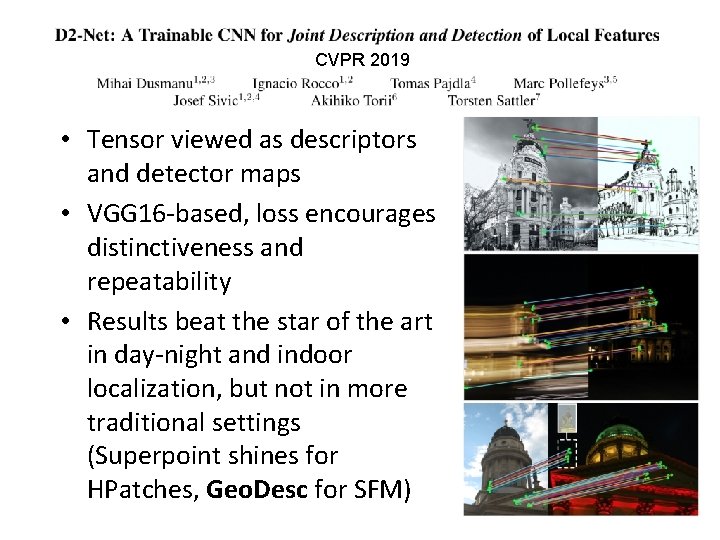
CVPR 2019 • Tensor viewed as descriptors and detector maps • VGG 16 -based, loss encourages distinctiveness and repeatability • Results beat the star of the art in day-night and indoor localization, but not in more traditional settings (Superpoint shines for HPatches, Geo. Desc for SFM)

Matching

Local features: main components 1) Detection: Identify the interest points 2) Description: Extract vector feature descriptor surrounding each interest point. 3) Matching: Determine correspondence between descriptors in two views Kristen Grauman

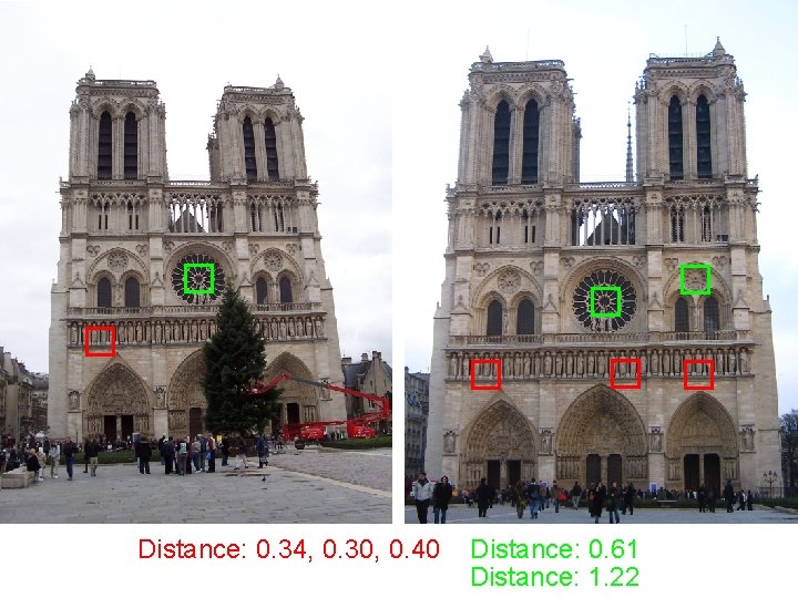
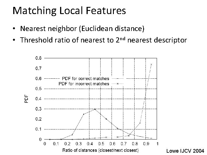
Matching • Simplest approach: Pick the nearest neighbor. Threshold on absolute distance • Problem: Lots of self similarity in many photos

Distance: 0. 34, 0. 30, 0. 40 Distance: 0. 61 Distance: 1. 22

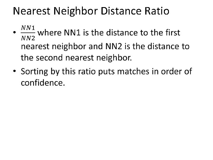
Nearest Neighbor Distance Ratio •

Matching Local Features • Nearest neighbor (Euclidean distance) • Threshold ratio of nearest to 2 nd nearest descriptor Lowe IJCV 2004

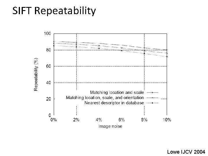
SIFT Repeatability Lowe IJCV 2004

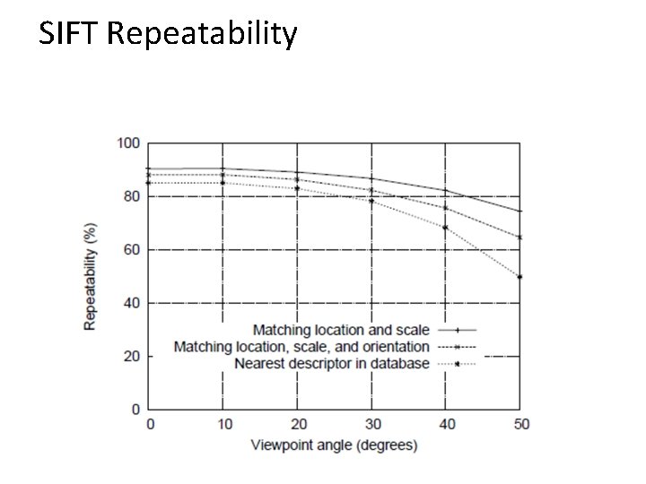
SIFT Repeatability