Descriptive Measures Descriptive Measure A Unique Measure of

Descriptive Measures Descriptive Measure – A Unique Measure of a Data Set 1) Central Tendency of Data A. Mean B. Median C. Mode 2) Dispersion or Spread of Data A. Range B. Quartiles & Percentiles C. Variance & Std Deviation

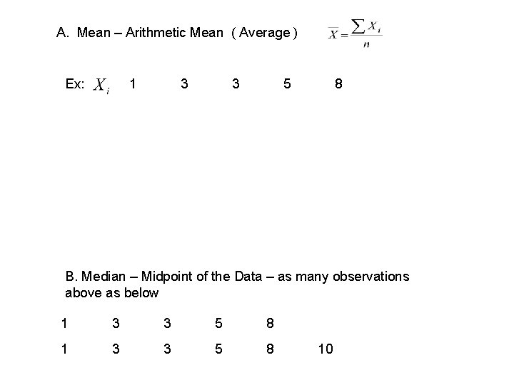
A. Mean – Arithmetic Mean ( Average ) Ex: 1 3 3 5 8 B. Median – Midpoint of the Data – as many observations above as below 1 3 3 5 8 10

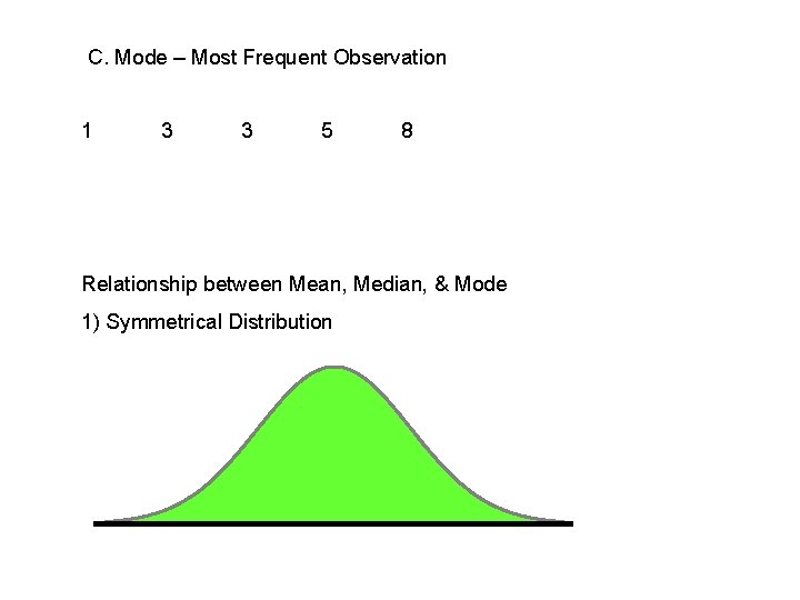
C. Mode – Most Frequent Observation 1 3 3 5 8 Relationship between Mean, Median, & Mode 1) Symmetrical Distribution

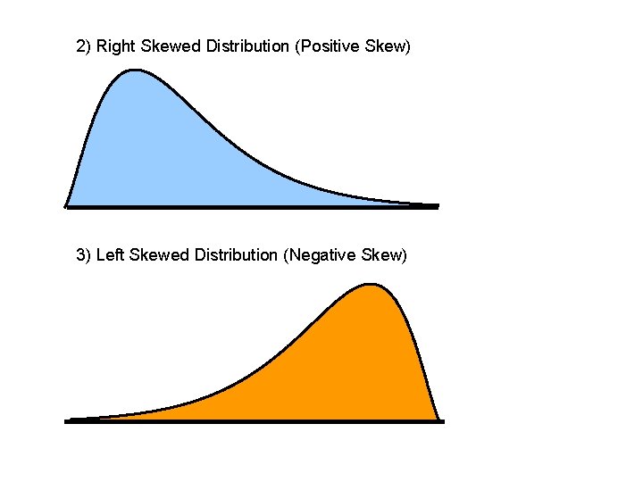
2) Right Skewed Distribution (Positive Skew) 3) Left Skewed Distribution (Negative Skew)

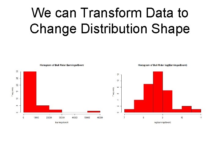
We can Transform Data to Change Distribution Shape

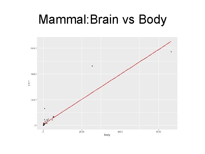
Mammal: Brain vs Body

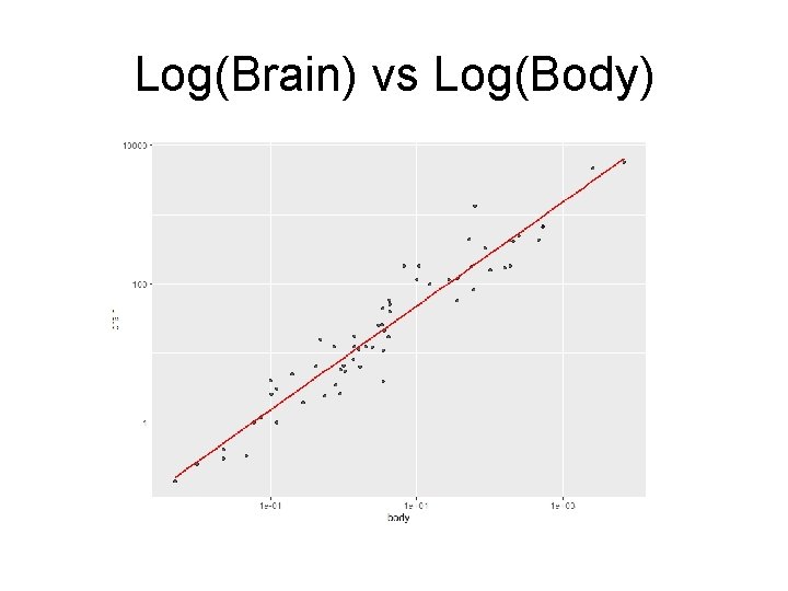
Log(Brain) vs Log(Body)

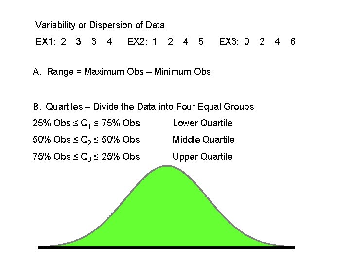
Variability or Dispersion of Data EX 1: 2 3 3 4 EX 2: 1 2 4 5 EX 3: 0 A. Range = Maximum Obs – Minimum Obs B. Quartiles – Divide the Data into Four Equal Groups 25% Obs ≤ Q 1 ≤ 75% Obs Lower Quartile 50% Obs ≤ Q 2 ≤ 50% Obs Middle Quartile 75% Obs ≤ Q 3 ≤ 25% Obs Upper Quartile 2 4 6

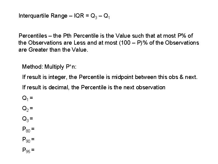
Interquartile Range – IQR = Q 3 – Q 1 Percentiles – the Pth Percentile is the Value such that at most P% of the Observations are Less and at most (100 – P)% of the Observations are Greater than the Value. Method: Multiply P*n: If result is integer, the Percentile is midpoint between this obs & next. If result is decimal, the Percentile is the next observation Q 1 = Q 2 = Q 3 = P 80 = P 95 =

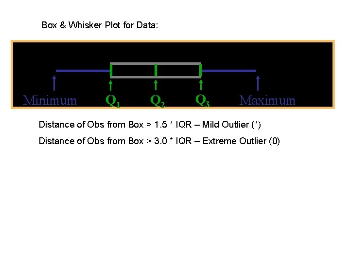
Box & Whisker Plot for Data: Minimum Q 1 Q 2 Q 3 Maximum Distance of Obs from Box > 1. 5 * IQR – Mild Outlier (*) Distance of Obs from Box > 3. 0 * IQR – Extreme Outlier (0)

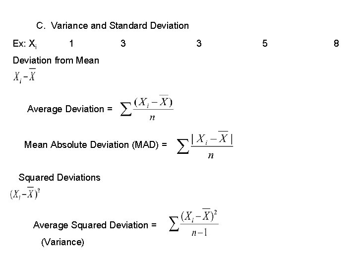
C. Variance and Standard Deviation Ex: Xi 1 3 Deviation from Mean Average Deviation = Mean Absolute Deviation (MAD) = Squared Deviations Average Squared Deviation = (Variance) 3 5 8

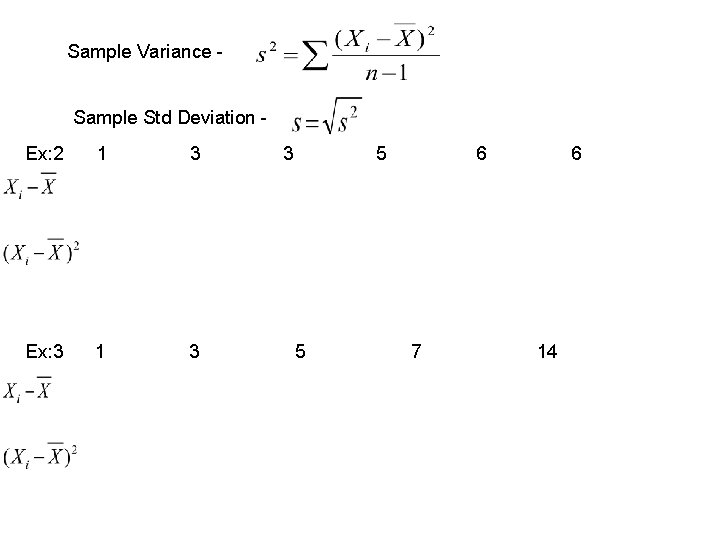
Sample Variance Sample Std Deviation Ex: 2 1 3 Ex: 3 1 3 3 5 5 6 7 6 14

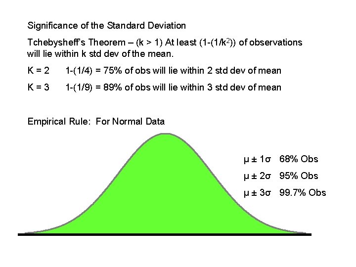
Significance of the Standard Deviation Tchebysheff’s Theorem – (k > 1) At least (1 -(1/k 2)) of observations will lie within k std dev of the mean. K=2 1 -(1/4) = 75% of obs will lie within 2 std dev of mean K=3 1 -(1/9) = 89% of obs will lie within 3 std dev of mean Empirical Rule: For Normal Data µ ± 1σ 68% Obs µ ± 2σ 95% Obs µ ± 3σ 99. 7% Obs

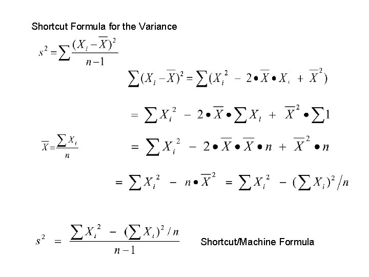
Shortcut Formula for the Variance Shortcut/Machine Formula

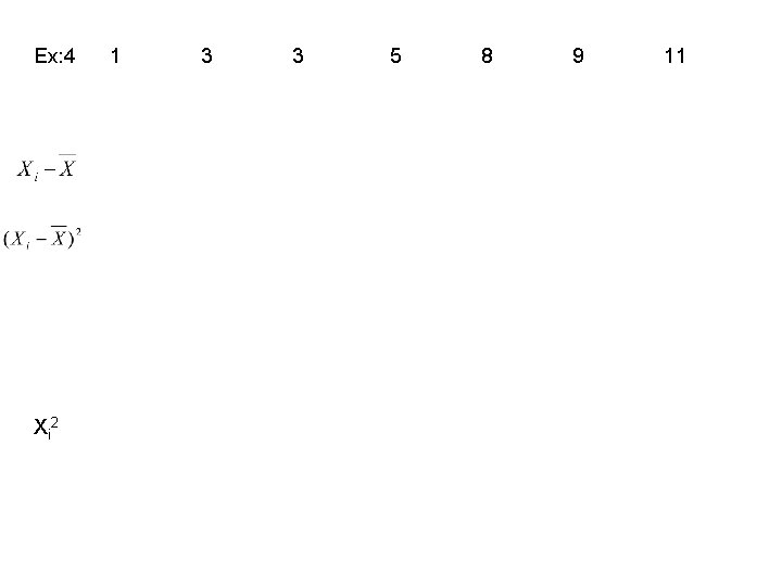
Ex: 4 Xi 2 1 3 3 5 8 9 11

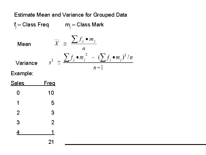
Estimate Mean and Variance for Grouped Data fj – Class Freq mj – Class Mark Mean Variance Example: Sales Freq 0 10 1 5 2 3 3 2 4 1 21

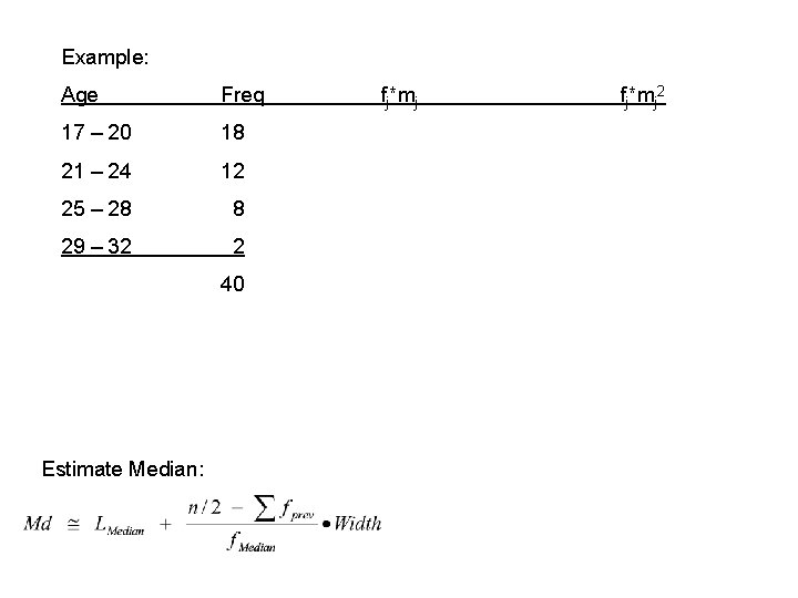
Example: Age Freq 17 – 20 18 21 – 24 12 25 – 28 8 29 – 32 2 40 Estimate Median: fj*mj 2

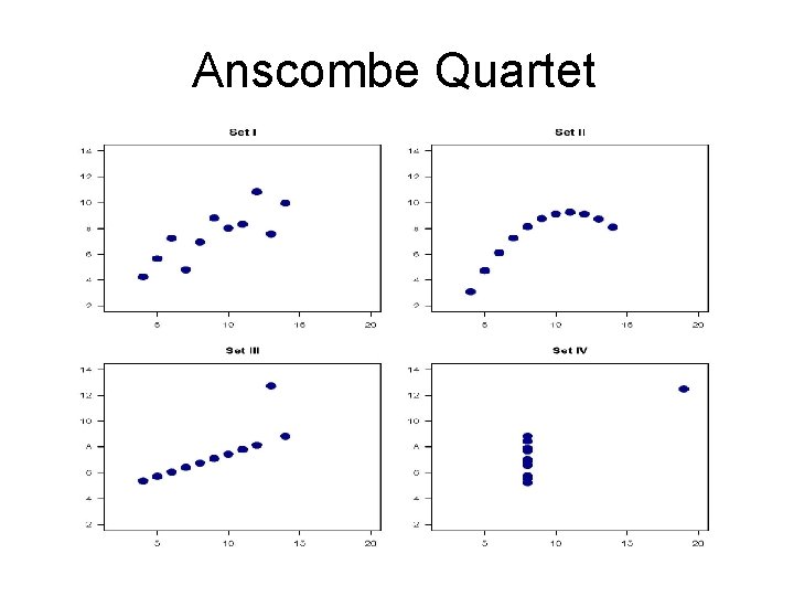
Anscombe Quartet