Describing Quantitative Distributions Descriptive Statistics 1 Summarizing Numerical

Describing Quantitative Distributions Descriptive Statistics 1
Summarizing Numerical Distributions � “SOCS” ◦ ◦ Shape (Distribution) Outliers Center Spread (Variation) � When on: examining a distribution visually, we want to mainly focus ◦ Shape ◦ Any unusual values (Potential Outliers) � We put less focus on but can roughly note: ◦ Typical Value (center) ◦ Variability (spread)
Characteristics of Shape � Is the distribution? ◦ Symmetric �Uniform �bell shaped ◦ Skewed �Left Skewed �Right skewed � Modality: How many mounds (or peaks) appear?
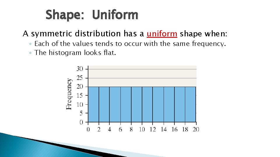
Shape: Uniform A symmetric distribution has a uniform shape when: ◦ Each of the values tends to occur with the same frequency. ◦ The histogram looks flat.
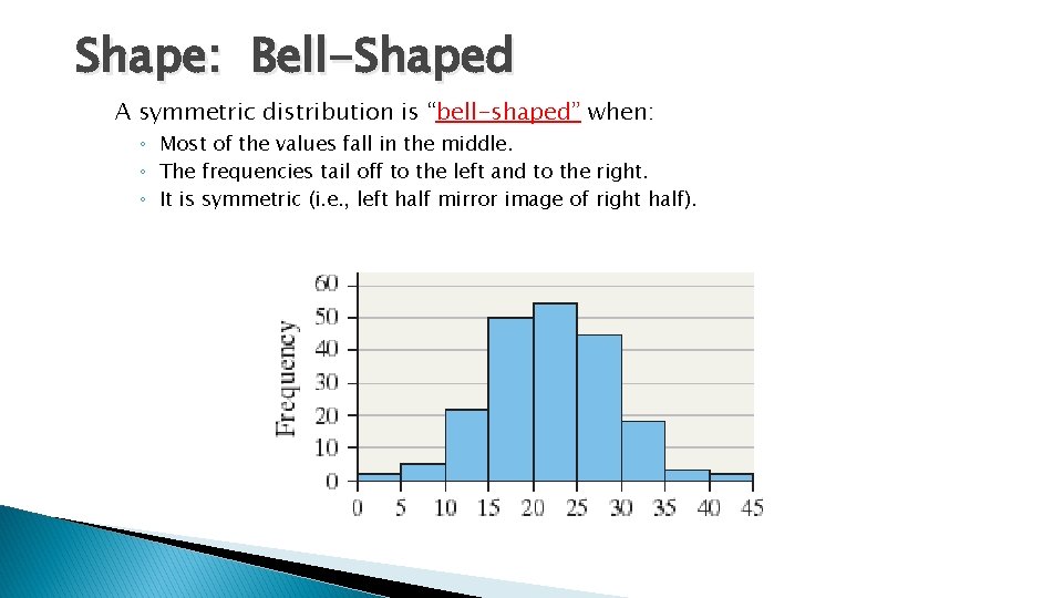
Shape: Bell-Shaped A symmetric distribution is “bell-shaped” when: ◦ Most of the values fall in the middle. ◦ The frequencies tail off to the left and to the right. ◦ It is symmetric (i. e. , left half mirror image of right half).

Right-Skewed Distribution A variable has a right-skewed distribution when: ◦ The “tail” extends out to the right. ◦ A few large values skew the distribution.
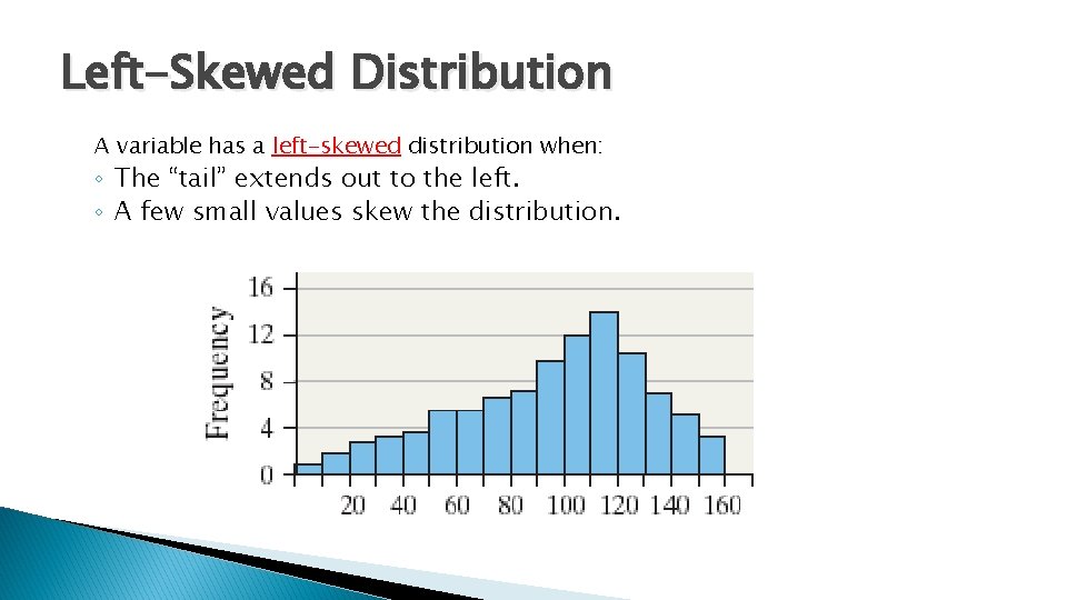
Left-Skewed Distribution A variable has a left-skewed distribution when: ◦ The “tail” extends out to the left. ◦ A few small values skew the distribution.
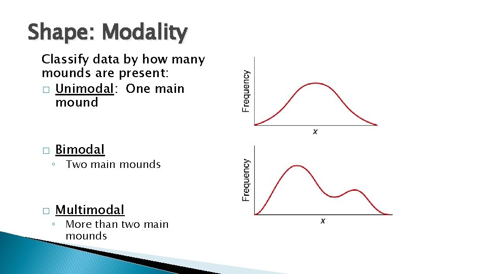
Shape: Modality Classify data by how many mounds are present: � Unimodal: One main mound � Bimodal ◦ Two main mounds � Multimodal ◦ More than two main mounds
Notes on Modality � Mounds can be different heights. � Bimodal and multimodal data may indicate existence of different groups within the data. � In this case, it may be preferable to separate the data into two groups and provide separate graphs for each group. � Examples: ◦ Men and women’s heights ◦ Afternoon and evening sales at a restaurant

Outliers � � Potential Outliers are: ◦ Extremely large or small values ◦ Do not fit the pattern of the rest of the data and ◦ May be apparent visually but subject to opinion. If ◦ ◦ ◦ you see extremely large or small values: Report the values. Realize they could be sources of error (typos, etc. ). Genuine outliers are unusually interesting data values

Center and Spread � Right now we are focusing on visual aspects and use rough measures of center and spread � Center: Best estimate of “Typical value” � Spread: Range of the data ◦ If the distribution is multimodal, we should note the multiple typical values.

Histogram Interpretation Example � What do you see? � Recall “SOCS” � Shape ◦ Symmetric ◦ Unimodal ◦ Bell-Shaped � Outliers ◦ Maybe a high outlier? � Center ◦ Between 110 -115. 114 ish? � Spread ◦ Range about = 135 -100 = 35 ish 12
Shape: Examples What shape would you expect to see in a histogram of the following data sets? � � GPA of college students ◦ Skewed left SAT scores ◦ Symmetric, Unimodal, Bellshaped Last digit of Social Security numbers for a random sample of students ◦ Symmetric, Uniform Income of USA residents ◦ Skewed right
- Slides: 13