Describing Distribution Numerically Center Median The middle number

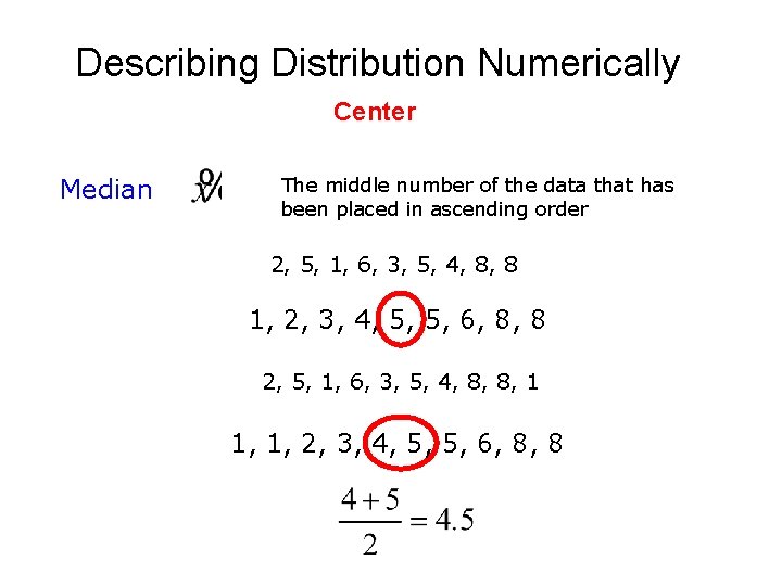
Describing Distribution Numerically Center Median The middle number of the data that has been placed in ascending order 2, 5, 1, 6, 3, 5, 4, 8, 8 1, 2, 3, 4, 5, 5, 6, 8, 8 2, 5, 1, 6, 3, 5, 4, 8, 8, 1 1, 1, 2, 3, 4, 5, 5, 6, 8, 8

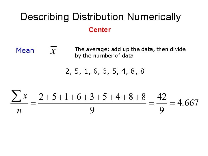
Describing Distribution Numerically Center Mean The average; add up the data, then divide by the number of data 2, 5, 1, 6, 3, 5, 4, 8, 8

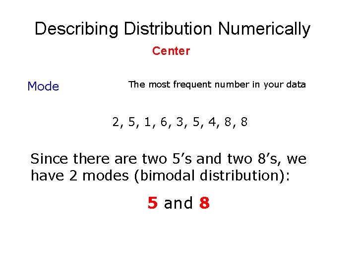
Describing Distribution Numerically Center Mode The most frequent number in your data 2, 5, 1, 6, 3, 5, 4, 8, 8 Since there are two 5’s and two 8’s, we have 2 modes (bimodal distribution): 5 and 8

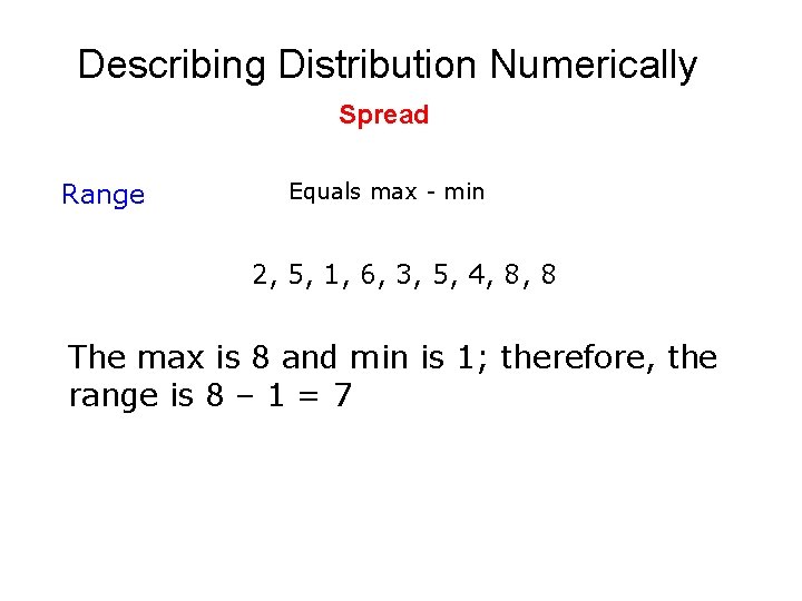
Describing Distribution Numerically Spread Range Equals max - min 2, 5, 1, 6, 3, 5, 4, 8, 8 The max is 8 and min is 1; therefore, the range is 8 – 1 = 7

Describing Distribution Numerically Spread Interquartile Range The data is placed in ascending order and split into quartiles (25%). (IQR) 2, 1, 5, 2, 1, 3, 6, 4, 3, 5, 5, 5, 4, 6, 8, 8, 8 8 25% 50% 75% Q 1 or QL Q 3 or QU IQR = Q 3 – Q 1 = 6 – 3 = 3 The middle 50% of the data will have a range of 3

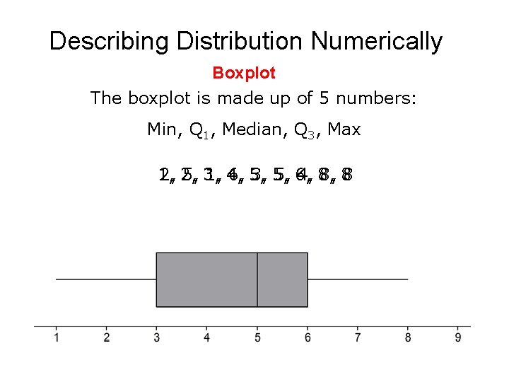
Describing Distribution Numerically Boxplot The boxplot is made up of 5 numbers: Min, Q 1, Median, Q 3, Max 1, 2, 2, 5, 3, 1, 4, 6, 5, 3, 5, 5, 6, 4, 8, 8, 8 8

Describing Distribution Numerically Standard Deviation The Standard Deviation determines how far the data is from the mean. If s is small, then the data is close to the mean. If s is large, then the data is spread out from the mean.

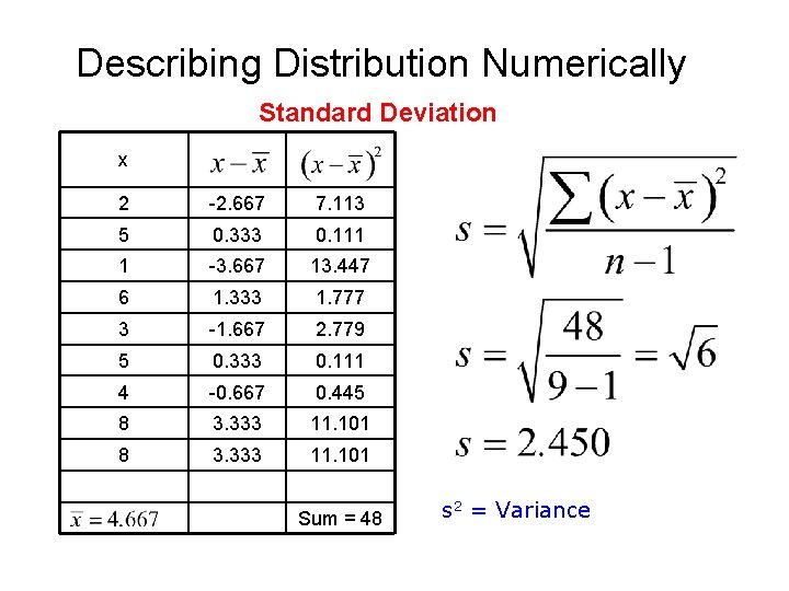
Describing Distribution Numerically Standard Deviation x 2 -2. 667 7. 113 5 0. 333 0. 111 1 -3. 667 13. 447 6 1. 333 1. 777 3 -1. 667 2. 779 5 0. 333 0. 111 4 -0. 667 0. 445 8 3. 333 11. 101 Sum = 48 s 2 = Variance

Announcements • According to Vox, the average restaurant meal is 4 times larger than in the 1950 s. • The i. Phone 7 WILL be released in black, according to Apple. • Ikea says that future homes will have vegetable planters lining their kitchen walls, furniture will double as exercise gear, and sensors throughout the house will respond instantly to our actions.

• Evens

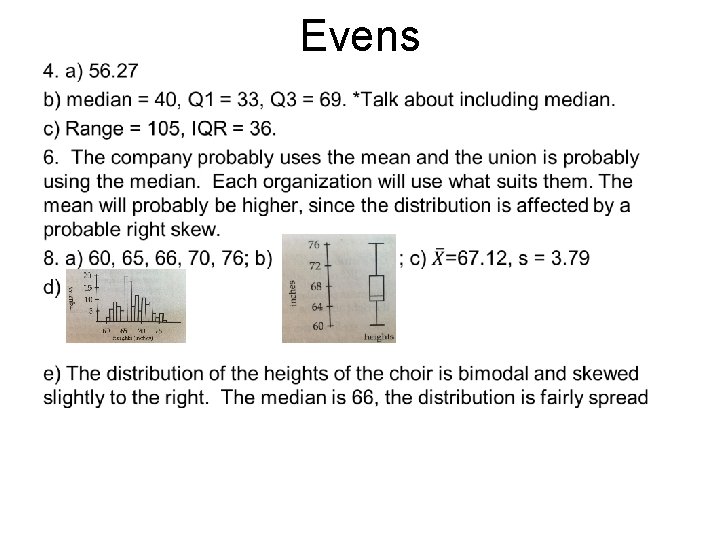
10. a) Set 2 has the greater standard deviation. Both sets have the same mean (7), maximum (10), and minimum (4), but 6 and 8 are farther from the mean than 7. s (set 1) = 2. 12, s (set 2) = 2. 24 b) Standard deviations are the same. Set 1 is the same as Set 2 +90. s (set 1) = 36. 06, s (set 2) = 36. 06. c) Set 2 has a greater standard deviation. The maximum and minimum of set 2 are farther away from the mean that of set 1. s (set 1) = 6. 03, s (set 2) = 7. 04. Pass up your homework!

Back to the notes from yesterday!

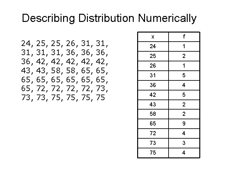
Describing Distribution Numerically 24, 31, 36, 43, 65, 73, 25, 31, 42, 43, 65, 72, 73, 25, 31, 42, 58, 65, 72, 75, 26, 36, 42, 58, 65, 72, 75, 31, 36, 42, 65, 65, 73, 75 x f 24 1 25 2 26 1 31 5 36 4 42 5 43 2 58 2 65 9 72 4 73 3 75 4

Describing Distribution Numerically Find the Mean, Standard Deviation, Q 1, Median, and Q 3

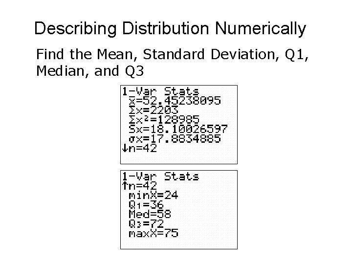
Describing Distribution Numerically Boxplots

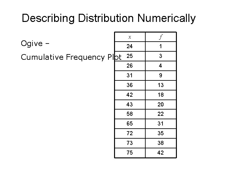
Describing Distribution Numerically Ogive – x f 24 1 Cumulative Frequency Plot 25 3 26 4 31 9 36 13 42 18 43 20 58 22 65 31 72 35 73 38 75 42

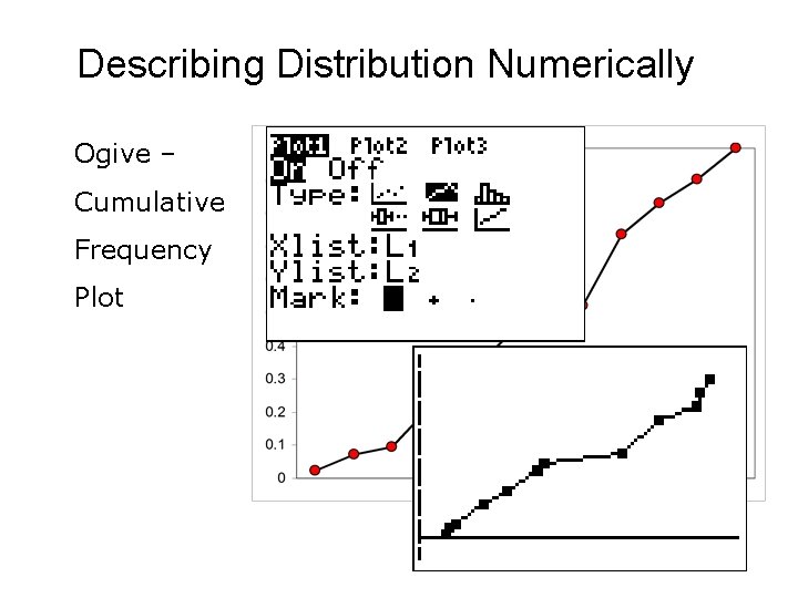
Describing Distribution Numerically Ogive – Cumulative Frequency Plot

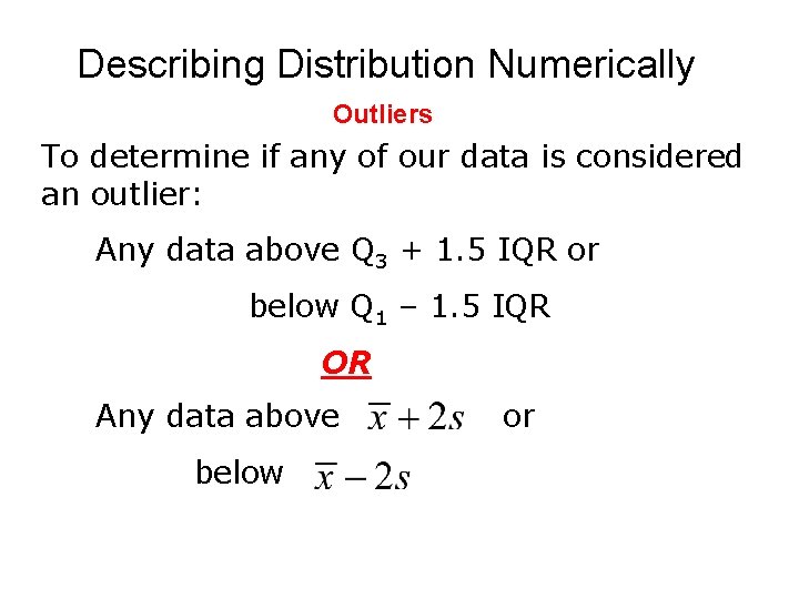
Describing Distribution Numerically Outliers To determine if any of our data is considered an outlier: Any data above Q 3 + 1. 5 IQR or below Q 1 – 1. 5 IQR OR Any data above below or

Describing Distribution Numerically Outliers 1, 2, 3, 4, 5, 5, 6, 8, 15 Q 1 Q 3 IQR = Q 3 – Q 1 = 6 – 3 = 3 Above Q 3 + 1. 5 IQR = 6 + 1. 5(3) = 10. 5 Below Q 1 – 1. 5 IQR = 3 - 1. 5(3) = -1. 5

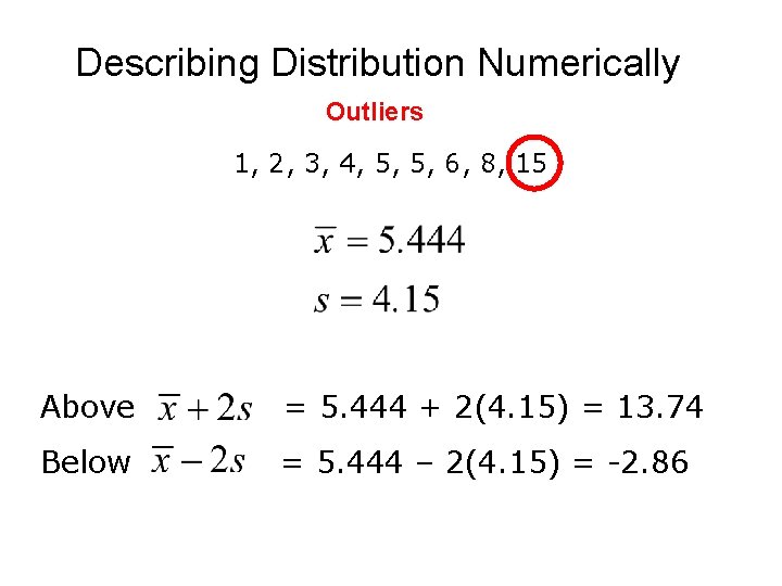
Describing Distribution Numerically Outliers 1, 2, 3, 4, 5, 5, 6, 8, 15 Above = 5. 444 + 2(4. 15) = 13. 74 Below = 5. 444 – 2(4. 15) = -2. 86

Describing Distribution Numerically Boxplots

Assignment Page 92: #12 – 23